Chapter 1: On Curves in General

Summary: Opening chapter of Book II. Euler sets up the geometric apparatus that will carry the rest of the volume: a variable quantity represented by a directed line, the abscissa/ordinate pair, orthogonal coordinates, and the basic taxonomy of curves (continuous vs. discontinuous, algebraic vs. transcendental, single- vs. multi-valued).

Sources: chapter1

Last updated: 2026-04-24

---

Overview

Book II is the geometric companion to Book I. Where Book I studied functions of a variable as analytic expressions, Book II asks how a function of $x$ becomes a curve in the plane, and conversely how a curve is read back as a function. This first chapter establishes the translation between the two — the coordinate apparatus — and then imports the Book I classifications (single/multi-valued, algebraic/transcendental, continuous/discontinuous) into the geometric setting.

Structure of the chapter

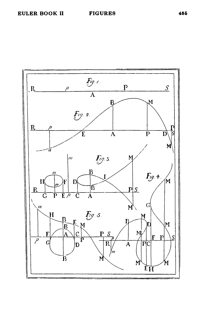
Paragraphs 1–3 represent a variable quantity $x$ by an indefinite straight line $RS$ with a chosen origin $A$; the abscissa $AP$ is cut off to the right for positive $x$ and to the left for negative $x$ (figure 1).

Paragraphs 4–8 extend the representation: a function $y$ of $x$ is pictured by erecting a perpendicular $PM$ (the ordinate) at each point $P$, above the axis when $y$ is positive and below when $y$ is negative. The locus of the extremities $M$ is the curve. “Thus any function of $x$ is translated into geometry and determines a line, either straight or curved” (source: chapter1, §6).

Paragraphs 9–10 introduce the Eulerian distinction between continuous and discontinuous curves: a continuous curve is one whose entire shape is captured by a single function of $x$; a discontinuous (also “mixed” or “irregular”) curve is one pieced together from different functions on different stretches. For the rest of Book II, “continuous” is the default object of study.

Paragraphs 11–14 fix the standard vocabulary: axis or directrix for the line $RS$, origin of the abscissas for the point $A$, abscissas for the intervals $AP$, ordinates for the perpendiculars $PM$. When the ordinate is perpendicular to the axis it is called orthogonal; otherwise oblique. The $(x,y)$ pair, when orthogonal, are the orthogonal coordinates (§14), and the curve is defined either by $y$ explicitly as a function of $x$ or by an equation in $x$ and $y$.

Paragraph 15 carries the Book I division into the geometric setting: a curve is [[algebraic-and-transcendental-curves|algebraic (also called geometric) or transcendental]] according as $y$ is an algebraic or a transcendental function of $x$.

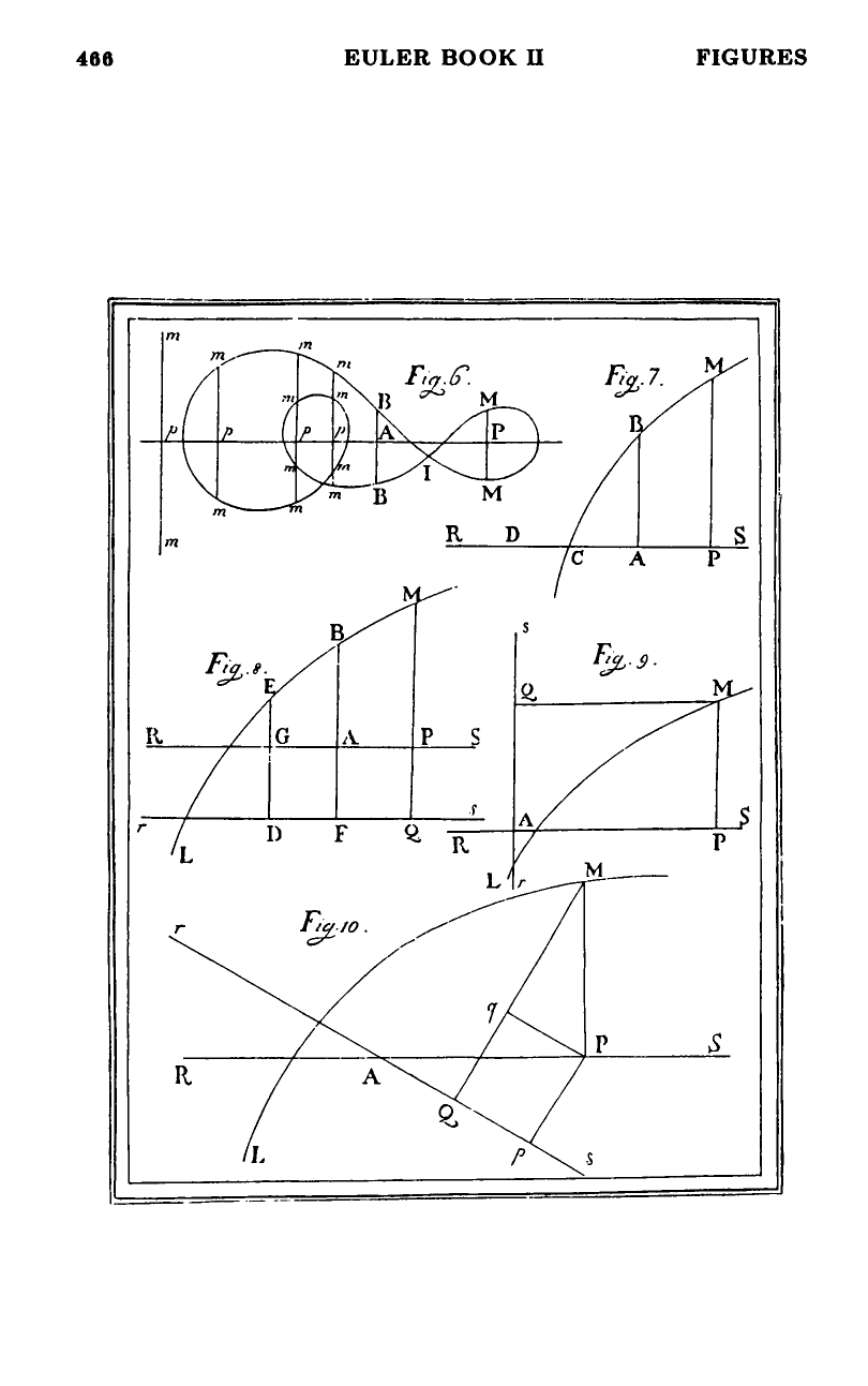
Paragraphs 16–22 treat multi-valued curves. A single-valued function produces a curve cut by each ordinate in exactly one point (figure 2). A two-valued function defined by $y^2=2Py-Q$ gives two ordinates per abscissa where $P^2>Q$, none where $P^2<Q$, and the curve “bends back” at the boundary $P^2=Q$ (figure 3). Three-valued (figure 4 or 5) and four-valued (figure 6) cases follow. The chapter closes with a parity principle: if one ordinate meets the curve in $m$ points, every other ordinate meets it in $m$, $m-2$, $m-4$, … points — the count is congruent to $m$ modulo 2 (§21). Consequently, the total number of branches extending indefinitely in both directions is always even, and if any ordinate cuts the curve oddly then every ordinate does (§22).

Notable points

• Euler’s “continuous” is not the modern $\epsilon$-$\delta$ notion. A modern piecewise-defined function with a kink — continuous in our sense — is “discontinuous” in his: the shape is not captured by one expression (source: chapter1, §9). See continuous-and-discontinuous-curves.
• A two-valued curve is not two curves. Its parts (e.g., $MBDBM$ and $FmHm$ in figure 3) “are to be considered as one continuous or regular curve, since all the different parts come from a single function” (source: chapter1, §18).
• Where the ordinate count drops from 2 to 0 — the boundary case $P^2=Q$ in §17 — the two real ordinates coalesce: $y=P\pm 0$. Geometrically the curve turns back on itself. This is Euler’s first brush with the idea of a turning point, before any calculus is available.
• Figure 6 (four-valued case, §20) already shows the possibility of a closed component: when neither side of the axis carries a branch to infinity, “the curve will be closed on both sides … and a definite area will be included” (source: chapter1, §20).
• The parity theorem of §21 is stated for curves defined by a polynomial equation in $y$ with single-valued coefficients. The argument is algebraic (complex roots come in pairs) rather than topological, but the conclusion is the same as the modern “asymptotic branches come in an even total” observation.

Why this chapter matters

This is where the Introductio turns from analysis to geometry. The Book I vocabulary is re-used wholesale — a curve’s nature is the function’s nature — so the reader is expected to carry over what they already know. What is new is the pictorial machinery: axes, abscissas, ordinates, branches. Every later chapter of Book II (conic sections, higher-degree curves, curvature, asymptotes, transcendental curves) is set in this frame.

Figures

Figures 1–5

Figures 6–10

Related pages

• abscissa-and-ordinate
• continuous-and-discontinuous-curves
• algebraic-and-transcendental-curves
• multi-valued-curves