Abscissa and Ordinate

Summary: The basic coordinate apparatus of Book II. The variable $x$ is represented by an interval $AP$ (the abscissa) cut off along a fixed line (the axis or directrix) from a chosen origin $A$; the value of a function $y$ of $x$ is represented by a perpendicular $PM$ (the ordinate) erected at $P$. The $(x,y)$ pair, when the ordinate is perpendicular to the axis, are the orthogonal coordinates.

Sources: chapter1

Last updated: 2026-04-24

---

From variable to interval (§§1–3)

A variable quantity is “a magnitude considered in general, and for this reason, it contains all determined quantities” (source: chapter1, §1). Euler represents such a magnitude by a straight line $RS$ of indefinite length, with a chosen point $A$ on it. A determined value of $x$ is then an interval $AP$ beginning at $A$:

• $P=A$ represents $x=0$;
• $P$ to the right of $A$ represents positive $x$, with farther-right meaning greater;
• $P$ to the left of $A$ represents negative $x$.

The choice of which direction is positive is arbitrary, but once chosen the opposite direction represents negative values (source: chapter1, §3). See figure 1.

From function to perpendicular (§§4–6)

Given $y$ a function of $x$, at each determined abscissa $AP$ the corresponding ordinate $PM$ is erected perpendicular to the axis — above the axis when $y>0$, below when $y<0$, and coincident with the axis (i.e., $M$ lies on $RS$) when $y=0$ (source: chapter1, §4). As $P$ sweeps along the axis, the locus of extremities $M$ is a line — straight or curved — called the curve of the function. “Thus any function of $x$ is translated into geometry and determines a line” (source: chapter1, §6).

Conversely, each point $M$ on the curve projects orthogonally to a unique $P$ on the axis, and so the curve is fully known once the function is known (source: chapter1, §7).

Standard vocabulary (§11)

Euler fixes the following terms, in use throughout Book II:

• axis or directrix: the line $RS$ along which $x$ is measured;
• origin of the abscissas: the point $A$ from which $x$ is measured;
• abscissa: the directed interval $AP$ representing a determined value of $x$;
• ordinate: the perpendicular $PM$ representing the corresponding value of the function $y$;
• orthogonal ordinate: the case when $PM\perp RS$; otherwise oblique ordinate.

“We will always explain the nature of curves with orthogonal ordinates unless we expressly indicate the contrary” (source: chapter1, §11).

Orthogonal coordinates and the equation of a curve (§§12–14)

When the ordinate is orthogonal, the pair $(x,y)$ is called the orthogonal coordinates (source: chapter1, §14). The curve is then defined in either of two equivalent ways:

• explicitly, by giving $y$ as a function of $x$, or
• implicitly, by an equation in $x$ and $y$ from which $y$ is determined by $x$.

Positive abscissas lie on the $AS$ part of the axis, negative on $AR$; positive ordinates above, negative below (source: chapter1, §12). To trace a curve from a given function, Euler (§13) sweeps $x$ from $0$ to $+\infty$ to build one part of the curve ($BMM$ in figure 2), then from $0$ to $-\infty$ for the other ($BEm$).

Relation to later chapters

This page pins down the vocabulary and reference frame; every subsequent chapter of Book II assumes it. The classification of curves by the kind of function $y$ is developed in algebraic-and-transcendental-curves and continuous-and-discontinuous-curves; the case where $y$ is not single-valued in $x$ is developed in multi-valued-curves.

Figures

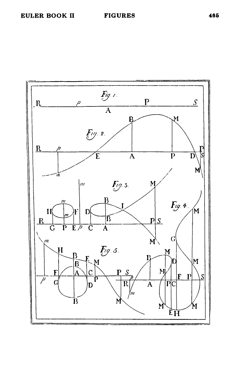Figures 1–5

Related pages

• chapter-1-on-curves-in-general
• continuous-and-discontinuous-curves
• algebraic-and-transcendental-curves
• multi-valued-curves