configuration-from-discriminant

Configuration from the Discriminant

Summary: Euler’s general method for reading the bounded-region shape of a curve whose equation is quadratic in the ordinate. Writing the equation as $y^2=(2Py-R)/Q$ with $P,Q,R$ polynomials in $x$, the polynomial $P^2-QR$ acts as a discriminant in $x$: its sign tells whether two ordinates are real, none are real, or two have collapsed to one. Real roots of $P^2-QR$ partition the axis into alternating real and complex intervals — the source of conjugate ovals — and coincident roots produce nodes, cusps, and conjugate points.

Sources: chapter12 (§§273–274, §§278–281, §283).

Last updated: 2026-05-04.

---

The setup

§280 — for any equation quadratic in $y$ the resolved form is

$$y=\frac{P\pm \sqrt{P^2-QR}}{Q},$$

with $P,Q,R$ polynomial in $x$. For each value of $x$:

• $P^2-QR>0$: two real ordinates.
• $P^2-QR<0$: no real ordinate (both complex).
• $P^2-QR=0$: a single ordinate $y=P/Q$ — the curve pinches to the axis-tangent direction or has a singular contact at this place.

The sign of the discriminant therefore controls everything that happens in the bounded region.

The interval picture

§280 — let ${\xi }_1<{\xi }_2<\cdots <{\xi }_m$ be the real roots of $P^2-QR$. They partition the $x$-axis into intervals on which $P^2-QR$ keeps a constant sign, alternating from one to the next. Every interval where the sign is positive carries a real two-valued arc of curve; every interval where the sign is negative carries no real points. The curve is the union of as many connected pieces as there are positive-sign intervals.

This is the source of the conjugate ovals. A pair of consecutive roots ${\xi }_i,{\xi }_{i+1}$ flanking a positive-sign interval produces an oval (or a finite arc closed by tangency at both ends if the discriminant has a double root somewhere); one bracketing a negative-sign interval traps a complex-only region between two real-arc regions.

The single-root scenario

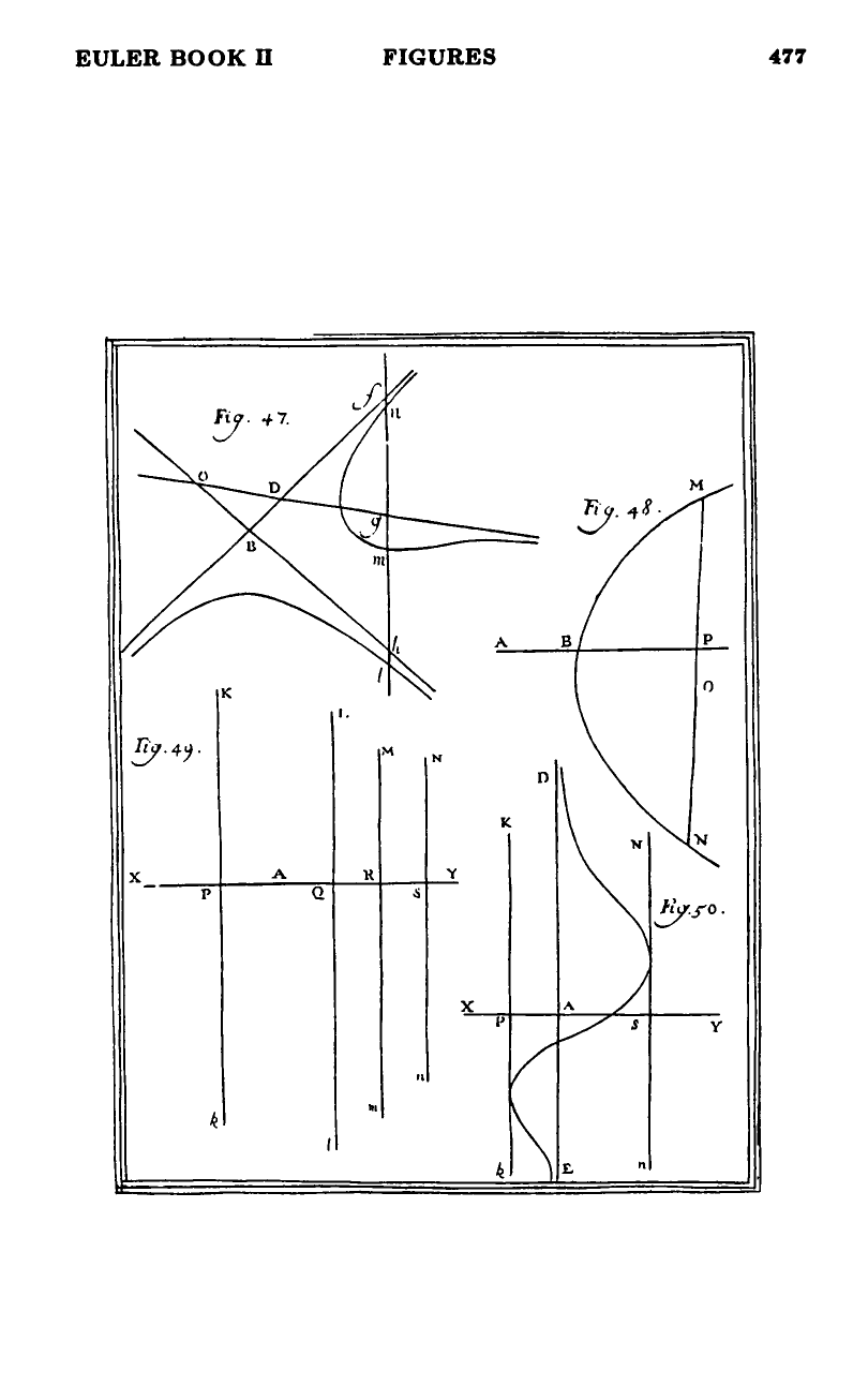
§§273–274 — the simplest non-trivial case is when the discriminant has only the leading even-degree term, so it goes negative in both directions far from the origin. There must then be at least two real roots. Two real roots $P,S$ enclose one real interval; outside it everything is complex and the curve is bounded between $x=P$ and $x=S$ (figures 49, 50). At $x=P$ and $x=S$ the two ordinates fuse, so the curve closes off there.

Outside the discriminant’s roots, “the ordinates become imaginary” — bounding the curve in the abscissa direction. This is Euler’s substitute for what would later be called the real-locus connectedness analysis.

Equal roots and singularities

§281 — collisions between consecutive roots of $P^2-QR$ collapse intervals.

Collision	Type of collapsed interval	Result
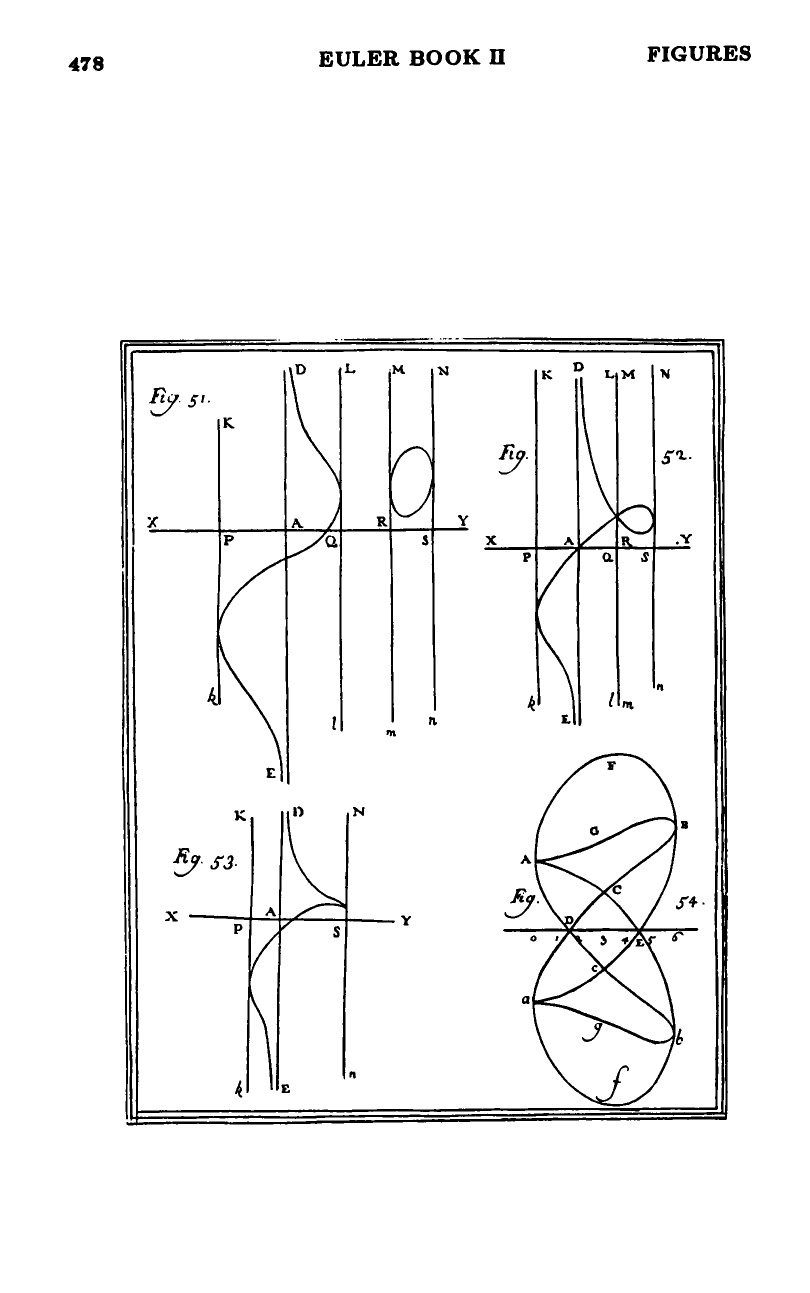
2 roots equal	positive-sign interval (real ordinates)	two ovals fuse → node (figure 52)
2 roots equal	negative-sign interval (complex ordinates)	conjugate oval shrinks to a single conjugate point
3 roots equal	adjacent +/−/+ shrinks	node tightens → cusp (figure 53)
4 roots equal	various	two separated ovals meet at a point; node grafted onto cusp; two cusps joined back-to-back
5 roots equal	—	cusp with two ovals attached; “almost nothing new”
more	—	no genuinely new configurations

See multiple-points-on-curves for the singular-point side of this dictionary; the present page focuses on the discriminant condition, that page on the local shape at the collision.

Linear and rational $y=P/Q$

§§278–279 — when one coordinate has degree one, $y=P/Q$ with $P,Q$ polynomial.

• $Q$ never vanishes ($P$ a polynomial): the curve is single-valued and tracks the axis to infinity in both directions.
• $Q$ has a simple real root at $x=f$: $y\to \pm \infty$ across $x=f$ with sign change — straight-line asymptote of species $u=A/t$.
• $Q$ has a double root $(x-f{)}^2$: $y$ keeps its sign across $x=f$ — asymptote of species $u^2=A/t$.
• $Q$ has a triple root $(x-f{)}^3$: sign-change again — like the simple case.

This is consistent with the chapter 7 and chapter 8 catalogue and is in fact the limiting case of the discriminant story when the radical degenerates.

Higher degree in $y$

§283 — when the equation is cubic, quartic, … in $y$, the number of real ordinates above each abscissa changes by 2, 4, 6, … at a time, and at every transition two real values fuse before they go complex (or a new pair appears from a fused state). Every such transition has the same local shape as one of the cases above. So a sample table of $y$-values at chosen $x$-values, with the sign-collisions noted, suffices to draw the curve. example-bounded-curve-eight-ordinates runs this on a curve with eight ordinates per abscissa.

Why this works

The discriminant analysis works because the curve, viewed as the real locus of a polynomial equation, can change topology only where the equation’s $y$-derivative vanishes (so two ordinates fuse) or where the leading $y$-coefficient vanishes (so a finite ordinate disappears to infinity). For a quadratic-in-$y$ equation, the first event is exactly the vanishing of $P^2-QR$ and the second is the vanishing of $Q$. Euler’s chapter is in effect a complete catalogue of the local pictures at both kinds of event.

Figures

Figures 47–50

Figures 51–54

Related pages

• chapter-12-on-the-investigation-of-the-configuration-of-curves — chapter summary.
• first-species-cubic-configurations — the §273–277 worked-out cubic case.
• multiple-points-on-curves — local shapes at coincident-root events.
• example-bounded-curve-eight-ordinates — §284 octic example.
• chapter-7-on-the-investigation-of-branches-which-go-to-infinity — the dual problem, where the polynomial side of $Q$‘s vanishing comes from.