First Species Cubic — Configurations

Summary: Euler unpacks the simplest first-species cubic from §258 into all its bounded-region varieties. Solved as a quadratic in the ordinate, the curve is governed by the quartic discriminant $b^2+dx+c{x}^2+a{x}^3-n^2{x}^4$. Two real factors give an asymptotic curve with a single curl (figure 50); four distinct real factors give the same plus a separate conjugate oval (figure 51); double, triple, etc. factors collapse the oval into a conjugate point, then graft it onto the curve as a node (figure 52), then tighten the node into a cusp (figure 53). Five varieties in all — Newton counted each as a different species, Euler counts them as one.

Sources: chapter12 (§§273–277). Figure 49 (in figures47-50); figure 50 (in figures47-50); figures 51, 52, 53 (in figures51-54).

Last updated: 2026-05-04.

---

The simplest first-species equation

§273 — from §258 (simplest-oblique-cubic-forms) the first cubic species has, in oblique coordinates $(t,u)$ with $u$ as abscissa and $t$ as ordinate, the form

$$y^2=\frac{2by+a{x}^2+cx+d-n^2{x}^3}{x},$$

a quadratic in $y$. Solving:

$$y=\frac{b\pm \sqrt{b^2+dx+c{x}^2+a{x}^3-n^2{x}^4}}{x},b\ne 0,n\ne 0.$$

The radicand is a quartic in $x$ with leading coefficient $-n^2<0$, so it is negative for $x\to \pm \infty$ and must have at least two real roots. Everything depends on how many real roots this quartic has.

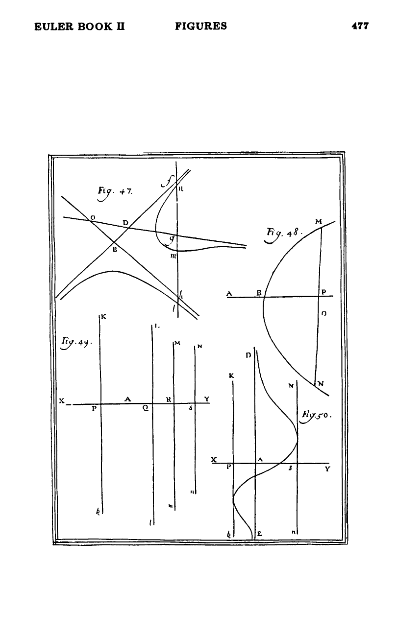
Variety 1 — two real roots (figure 50)

§§274–275 — the radicand has only two real roots, $P$ and $S$. On the open interval $(P,S)$ both ordinates are real; outside it both are complex. So the curve lies entirely between the two vertical lines $x=P$ and $x=S$ in figure 49 (which sets up the labelling: vertical lines $Kk,Ll,Mm,Nn$ through points $P,Q,R,S$ on the axis).

Where does the curve do at the origin? The denominator is $x$, so $x=0$ is an asymptotic vertical line. But the numerator also has a determined behavior: at $x=0$,

$$\sqrt{b^2+dx+\cdots }\approx b+\frac{dx}{2b},$$

so

$$y=\frac{b\pm (b+dx/(2b))}{x}=\{\begin{array}{ll}\frac{2b}{x}+\frac{d}{2b}\to \infty & (+\text{ branch})\\ -\frac{d}{2b}& (-\text{ branch}).\end{array}$$

So the $+$ branch goes to infinity along the $y$-axis (the $y$-axis is an asymptote), but the $-$ branch passes through the finite point $(0,-d/(2b))$. The curve is the S-shape of figure 50: an asymptotic branch hugging the $y$-axis from below, swinging across through the point $(0,-d/(2b))$, and looping over to a tangential closure at $x=S$ on the right.

Variety 2 — four distinct real roots; conjugate oval (figure 51)

§276 — when the discriminant has four distinct real roots $P<Q<R<S$, the sign of $b^2+dx+c{x}^2+a{x}^3-n^2{x}^4$ alternates: positive on the central interval $(Q,R)$ no — wait — the leading coefficient is $-n^2<0$, so the sign pattern from $-\infty$ to $+\infty$ is $-+-+-$. The two positive intervals are $(P,Q)$ and $(R,S)$. The curve lives over both of them.

Over $(P,Q)$: real two-valued arc, closed off at $x=P$ and $x=Q$ by tangential collapse — an oval bounded by vertical lines $Kk$ and $Ll$.

Over $(R,S)$: another real two-valued arc — an oval bounded by $Mm$ and $Nn$.

The origin $A$ is between two of the four roots (Euler argues: since both ordinates at $x=0$ are real, $A$ lies in $(P,Q)$ or in $(R,S)$). The asymptote at $x=0$ now joins one of the two arcs into the figure-50-style asymptotic curl. The other arc is left over as a self-contained oval, separated from the asymptotic branch:

“The curve consists of two parts which are separated; one lies between the straight lines $Kk$ and $Ll$, while the other lies between the straight lines $Mm$ and $Nn$. … In this case the curve has the configuration shown in figure 51, called a CONJUGATE OVAL, that is, it consists of an oval, called a conjugate oval, separated from the rest of the curve which is related to the asymptote $DE$.”

This is the first appearance in the chapter of the term conjugate oval.

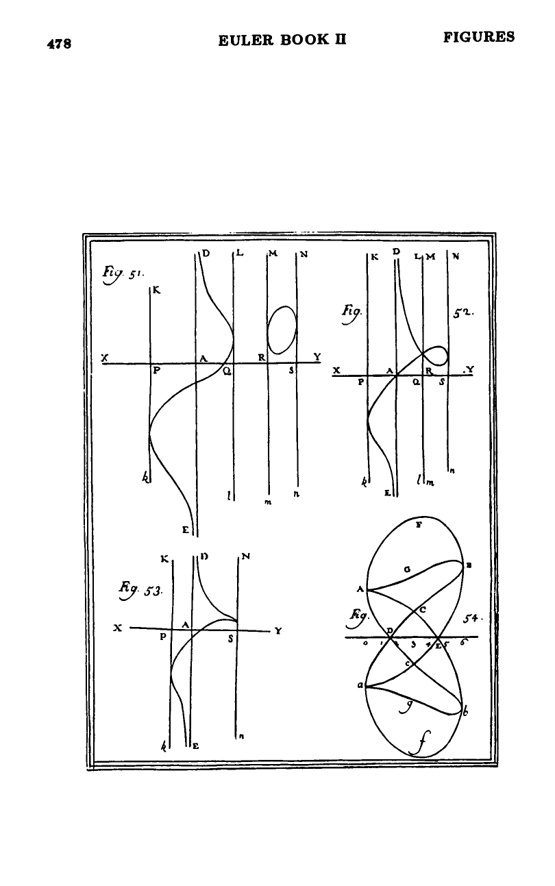
Variety 3 — conjugate point ($R$ and $S$ coincide)

§277 — let two of the four roots merge.

• $P=Q$? Impossible: $A$ lies between $P$ and $Q$ and would have to satisfy both roots, forcing $b=0$, contradicting the assumption $b\ne 0$.
• $R=S$: the conjugate oval shrinks to nothing — its vertical extent collapses because the two tangential closures fuse. What remains is a single isolated point lying on the axis at $x=R=S$. This is the conjugate point (point isolé): a real solution of the equation that is not connected to any real arc. The picture is figure 50 plus an isolated dot on the axis.

Variety 4 — node ($Q$ and $R$ coincide; figure 52)

§277 — when the two interior roots merge, $Q=R$, the negative-sign interval $(Q,R)$ between the two real-ordinate arcs disappears. The two arcs no longer separate: they touch at the common point $x=Q=R$ on the axis. The asymptotic curl now has the conjugate oval grafted onto it through a single shared point. The two arcs cross transversally at this point, since the discriminant has only a simple zero of multiplicity 2 there (not a triple zero). This is a node — also called a double point (see multiple-points-on-curves). Figure 52 shows the configuration: the figure-50 curve has acquired a self-intersecting loop at the right.

Variety 5 — cusp ($Q,R,S$ all coincide; figure 53)

§277 — when three of the roots merge, $Q=R=S$, the loop of figure 52 tightens further: the two formerly separate ovals are joined not just at a transversal crossing but at a tangential one. This is a cusp (figure 53): the loop has shrunk to a single sharp point on the axis, with the two arcs of the curve approaching from opposite directions but along a common tangent.

Summary table

#	Discriminant roots	Configuration	Figure
1	$P,S$ (2 real)	asymptotic curl (no oval)	50
2	$P,Q,R,S$ all distinct	curl + conjugate oval	51
3	$P,Q,R=S$	curl + conjugate point	(50 plus isolated point)
4	$P,Q=R,S$	curl with node	52
5	$P,Q=R=S$	curl with cusp	53

“Hence there are five different varieties which find a place in the first species. Newton considered each of these to be a different species.” (§277)

This is one of the chapter’s two big editorial points (the other being the multiple-points classification, §282): the 72-vs-16 ratio between Newton and Euler in cubic species is doing exactly this kind of bookkeeping inside each of Euler’s species, which is why it inflates the count.

§278 — extension to the other cubic species

The same approach handles the other 15 species. Wherever one coordinate appears with degree no greater than 2, the discriminant-of-a-quadratic-in-$y$ argument applies. Euler does not enumerate this in detail; the chapter then turns to the general method and the singular-point classification that systematizes what these worked cases illustrate.

Figures

Figures 47–50

Figures 51–54

Related pages

• chapter-12-on-the-investigation-of-the-configuration-of-curves — chapter summary.
• configuration-from-discriminant — the general method this case instantiates.
• multiple-points-on-curves — node, cusp, conjugate point as a separate concept page.
• simplest-oblique-cubic-forms — §258, source of the equation worked out here.
• cubic-species-classification — the species this is the simplest of.
• euler-vs-newton-cubic-species — Newton’s “5 species” choice vs. Euler’s “5 varieties of one species” choice.