Curvilinear Asymptote Refinement

Summary: The master move of chapter-8-concerning-asymptotes. Given a straight-line asymptote $u=c$ produced by a simple real linear factor $ay-bx$ of the highest member $P$, refine it to a curvilinear asymptote that approximates the original curve more closely. The procedure: rotate axes onto the asymptote direction, expand $P+Q+R+\cdots =0$ in descending powers of $t$ with coefficients in $u$, substitute $u=c$ everywhere except in the term that vanishes when $u=c$, and read off a sequence of refinements $(u-c)+A/t^k=0$ for $k=1,2,\dots ,n-1$. The first non-vanishing $A$ tells how fast and on which side the curve approaches $u=c$.

Sources: chapter8 (§§200–203), figures35-39 (figures 35, 36, 37).

Last updated: 2026-04-28

---

Setup: rotate onto the asymptote direction

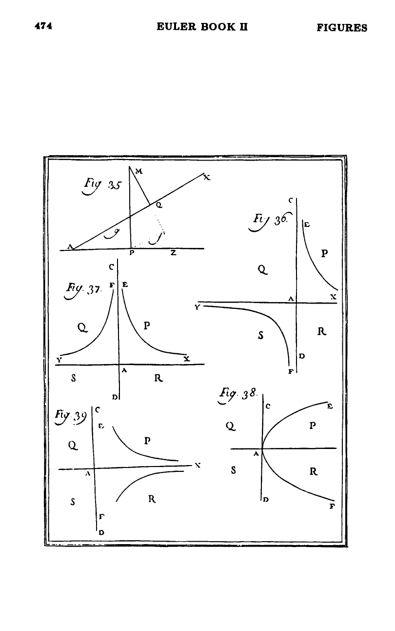
§200. Suppose $P=(ay-bx)M$ where $M$ is homogeneous of degree $n-1$ and not divisible by $ay-bx$. Let $AZ$ be the original abscissa axis with $AP=x$, $PM=y$ (figure 35). Choose a new axis $AX$ through the origin $A$ at angle $\arctan (b/a)$ to $AZ$ — the direction of the asymptote. So

$\sin \angle XAZ=\frac{b}{\sqrt{a^2+b^2}},\cos \angle XAZ=\frac{a}{\sqrt{a^2+b^2}}.$

On the new axis, take abscissa $AQ=t$ and ordinate $QM=u$. With $g=\sqrt{a^2+b^2}$, the new and old coordinates relate by

$t=\frac{ax+by}{g},u=\frac{ay-bx}{g},y=\frac{au+bt}{g},x=\frac{at-bu}{g}.$

So $u$ — the new ordinate — is, up to the constant $g$, the very factor $ay-bx$ of $P$. The straight-line asymptote will become a horizontal line $u=c$.

Member expansion in $(t,u)$

§201. Substitute $y=(au+bt)/g$, $x=(at-bu)/g$ into $P+Q+R+S+\cdots =0$ and group by powers of $t$. The members take the schematic form (relabelling coefficients $\alpha ,\beta ,\gamma ,\delta ,ϵ,\dots$ for cleanliness):

$M=\alpha t^{n-1}+\alpha t^{n-2}u+\alpha t^{n-3}{u}^2+\cdots ,$ $Q=\beta t^{n-1}+\beta t^{n-2}u+\beta t^{n-3}{u}^2+\cdots ,$ $R=\gamma t^{n-2}+\gamma t^{n-3}u+\gamma t^{n-4}{u}^2+\cdots ,$ $S=\delta t^{n-3}+\delta t^{n-4}u+\delta t^{n-5}{u}^2+\cdots ,$ $T=ϵt^{n-4}+ϵt^{n-5}u+ϵt^{n-6}{u}^2+\cdots ,$

and so on. (The recycled letters refer to different coefficients in each member.) Note that $P=uM$ at this stage, so $P$ contributes $\alpha t^{n-1}u+\alpha t^{n-2}{u}^2+\cdots$; multiplied by $u$, the $M$-coefficients land one column to the left.

As $t\to \infty$, in any given member only the first non-vanishing term survives; subsequent terms in the same member are smaller by a factor of $u/t$ (which tends to zero on a branch approaching the asymptote $u=c$, since $u$ stays bounded while $t\to \infty$).

The straight-line asymptote (§202)

Since $M$ is not divisible by $u$, its first term is present: $M$ starts with $\alpha t^{n-1}$. So $P=uM$ starts with $\alpha t^{n-1}u$, and $Q$ starts with $\beta t^{n-1}$. The leading equation at infinity is

$\alpha t^{n-1}u+\beta t^{n-1}=0⟹u=-\frac{\beta }{\alpha }=:c.$

This is the straight-line asymptote: the line $u=c$ parallel to and at distance $c$ from the new axis $AX$.

Refinement: substitute $u=c$ everywhere except in the leading term

§202. To find a closer-fitting curvilinear asymptote, set $u=c$ in every member except the term $\alpha t^{n-1}u$ — the term that records the deviation $u-c$. The equation reduces to

$\alpha t^{n-1}u+\beta t^{n-1}+t^{n-2}(\alpha c^2+\beta c+\gamma )+t^{n-3}(\alpha c^3+\beta c^2+\gamma c+\delta )+\cdots =0.$

Using $\alpha u+\beta =\alpha (u-c)$ to factor out $u-c$:

$\alpha (u-c)t^{n-1}+t^{n-2}(\alpha c^2+\beta c+\gamma )+t^{n-3}(\alpha c^3+\beta c^2+\gamma c+\delta )+\cdots =0.$

Divide by $\alpha t^{n-1}$:

$(u-c)+\frac{A_1}{t}+\frac{A_2}{t^2}+\cdots +\frac{A_{n-1}}{t^{n-1}}=0$

where $A_k=(\alpha c^{k+1}+\beta c^k+\gamma c^{k-1}+\cdots )/\alpha$.

Reading off the refinement. Truncate at the first non-vanishing coefficient. Denote it $A$ and its position $k$:

• If $A_1\ne 0$: refinement is $(u-c)+A/t=0$.
• If $A_1=0$ but $A_2\ne 0$: refinement is $(u-c)+A/t^2=0$.
• Generally: $(u-c)+A/t^k=0$ for the smallest $k$ with $A_k\ne 0$.
• If $A_1=A_2=\cdots =A_{n-1}=0$: then the equation becomes $(u-c)\cdot \alpha t^{n-1}=0$, meaning $u-c$ divides the original polynomial. The straight line $u=c$ is then part of the curve — the curve is reducible (see complex-curves).

Canonical form $z=C/t^k$ (§203)

Setting $z=u-c$ — choosing the asymptote line itself as the new axis $XY$ (figure 36) — every refined asymptote takes the form

$z=\frac{C}{t^k},1\le k\le n-1.$

The four quadrants formed by $XY$ (the asymptote, horizontal) and the perpendicular line $CD$ at the origin $A$ are labelled $P,Q,R,S$ counterclockwise from upper-right (figure 36).

Parity rule for the quadrant pattern

The shape depends on the parity of $k$:

• $k$ odd (e.g. $z=C/t$): $z$ has the same sign as $C/t^k$, which flips with the sign of $t$. Two branches $EX$ in quadrant $P$ ($t>0$, $z>0$ if $C>0$) and $FY$ in quadrant $S$ ($t<0$, $z<0$). Branches lie in opposite quadrants — figure 36.
• $k$ even (e.g. $z=C/t^2$): $z$ has the fixed sign of $C$ regardless of $t$. Two branches $EX$ and $FY$ both above (if $C>0$) or both below (if $C<0$) the asymptote, in adjacent quadrants $P$ and $Q$ — figure 37.

The convergence is faster for larger $k$: $z\to 0$ as $1/t^k$, so the curve hugs the asymptote more tightly.

What’s gained over the straight line alone

The straight-line asymptote $u=c$ tells you the limiting direction and limiting position. The curvilinear refinement $u-c=A/t^k$ additionally tells you:

1. The side of approach. Sign of $A$ (and parity of $k$) decides whether the branch is above or below the line, and whether the two branches lie on the same side or opposite sides.
2. The rate of approach. The exponent $k$: $k=1$ is “hyperbolic” (slow); larger $k$ is faster.
3. Whether the branches cross the line. Only the parity of $k$ together with the sign $C/t^k$ can flip — but $u-c=A/t^k$ never crosses $u=c$ for finite $t$, only at $t=\infty$.

This gives qualitative information — quadrant pattern, side, rate — that the straight-line asymptote cannot encode.

Worked structure

The refinement is mechanical once the rotation is in place:

1. Compute $\alpha =M(b,a)$ and $\beta =Q(b,a)$ (substitute $y=b,x=a$ into the coefficients of the dominant terms in $M$ and $Q$). The asymptote is $u=c$ with $c=-\beta /\alpha$.
2. Compute $A_1=(\alpha c^2+\beta c+\gamma )/\alpha$. If non-zero, the refinement is $(u-c)+A_1/t=0$.
3. If $A_1=0$, compute $A_2=(\alpha c^3+\beta c^2+\gamma c+\delta )/\alpha$. If non-zero, the refinement is $(u-c)+A_2/t^2=0$.
4. Continue until the first non-vanishing $A_k$ is found.

Figures

Figures 35–39

Related pages

• chapter-8-concerning-asymptotes
• rectilinear-asymptote-from-equation
• branches-at-infinity
• double-factor-asymptote-cases
• triple-factor-asymptote-cases
• hyperbolic-and-parabolic-branches
• curvilinear-asymptote
• complex-curves