example-curve-eight-branches

Example: Eight-Branch Curve $y^3{x}^2(y-x)-xy(y^2+x^2)+1=0$

Summary: Euler’s worked example closing chapter 8. The sextic curve $y^3{x}^2(y-x)-xy(y^2+x^2)+1=0$ has principal member $P=y^3{x}^2(y-x)$, which factors with three different multiplicities — single $(y-x)$, double $x^2$, triple $y^3$ — exercising in one curve every case from §§200–214. Each factor is treated by the chapter’s refinement procedure: the single factor produces a hyperbolic-rate curvilinear asymptote $y-x=2/x$ along the line $y=x$ (2 branches); the double factor produces a parabolic-rate asymptote and a pair of $u=1/t^3$ asymptotes along the $y$-axis (4 branches); the triple factor produces a single $u=1/t^3$ asymptote along the $x$-axis (2 branches). Total: 8 branches at infinity, drawn as figure 43.

Sources: chapter8 (§§215–217), figures40-43 (figure 43).

Last updated: 2026-04-28

---

The curve

§215. The given equation is

$y^3{x}^2(y-x)-xy(y^2+x^2)+1=0.$

The principal member (highest member, degree 6) is $P=y^3{x}^2(y-x)$. Its real-linear-factor decomposition is

$P=(y-x)\cdot x^2\cdot y^3,$

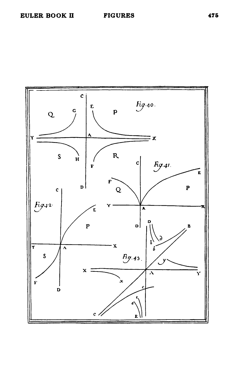
three different real factors with multiplicities $1,2,3$. By branches-at-infinity, each contributes branches at infinity; by curvilinear-asymptote-refinement, double-factor-asymptote-cases, and triple-factor-asymptote-cases, the asymptote shapes are read off in turn. The curve has, in total, 8 branches going to infinity, displayed as figure 43.

Single factor $y-x$ (§215, simple-factor case)

The factor $y-x$ has multiplicity 1, so this is a curvilinear-asymptote-refinement / rectilinear-asymptote-from-equation case.

Quick refinement. Since $y-x$ is a single factor, isolate it from the equation and substitute $y=x$ in the remainder. From $y^3{x}^2(y-x)-xy(y^2+x^2)+1=0$, solve for $y-x$:

$y-x=\frac{xy(y^2+x^2)-1}{y^3{x}^2}=\frac{(y^2+x^2)}{y^{2}x}-\frac{1}{y^3{x}^2}.$

Substitute $y=x$ in the right-hand side:

$y-x=\frac{2x^2}{x^3}-\frac{1}{x^5}=\frac{2}{x}-\frac{1}{x^5}.$

At infinity ($x=\infty$) the second term vanishes faster, leaving

$y-x=\frac{2}{x},$

i.e. straight-line asymptote $y=x$ refined to curvilinear asymptote $y-x=2/x$.

Geometric placement. The straight-line asymptote $y-x=0$ is the line $BAC$ in figure 43 — the diagonal making an angle of $45°$ (half a right angle) with the original axis $XY$, through the origin $A$.

Coordinate change to the asymptote axis. To verify and study the branches, rotate axes onto the asymptote direction. Set $a=b=1$, $g=\sqrt{2}$, so

$y=\frac{u+t}{\sqrt{2}},x=\frac{t-u}{\sqrt{2}}.$

Substituting into the equation:

$\frac{(u+t)(t^2-u^2)u}{4}+\frac{(t^2-u^2)(t^2+u^2)}{2}+1=0$

(after collecting and using $y^3{x}^2(y-x)=(u+t{)}^3(t-u{)}^2(-2u)/(4\sqrt{2})$… Euler’s expansion). Multiplying by 4 and reorganising:

$0=t^{5}u+t^4{u}^2-2t^3{u}^3-2t^2{u}^4+t{u}^5+u^6-2t^4+2u^4+4.$

At $t=\infty$ with $u\to 0$, only the terms $t^{5}u-2t^4$ avoid vanishing. The leading equation is

$t^{5}u-2t^4=0⟹u=\frac{2}{t}.$

This is the curvilinear asymptote $u=2/t$ along the diagonal $BAC$ — a hyperbolic-rate refinement, $k=1$ in the curvilinear-asymptote-refinement catalogue. By the parity rule (§203), $k=1$ odd → branches in opposite quadrants of the asymptote. Two branches $bB$ and $cC$ in figure 43, on opposite sides of $BAC$.

Double factor $x^2$ (§216, double-factor case)

The factor $x^2$ has multiplicity 2, so this is a double-factor-asymptote-cases case. The asymptote direction is the vertical — perpendicular to the $XY$ axis — so the new axis is $AD$ in figure 43.

Set $y=t$, $x=u$ (the new abscissa is along $AD$, the original $y$-axis; the new ordinate is along the original $x$-axis). The equation becomes

$0=t^4{u}^2-t^3{u}^3-t^{3}u-t{u}^5+1.$

(One can derive this directly: $y^3{x}^2(y-x)=t^4{u}^2-t^3{u}^3$, $-xy(y^2+x^2)=-t^{3}u-t{u}^3$ — but the cross-term $-t{u}^3$ has lower degree than $-t{u}^5$ at infinity, so on Euler’s normalisation it goes into the higher-power category. Euler’s printed form is the expansion above.)

At $t=\infty$ the leading equation is

$t^4{u}^2-t^{3}u+1=0,$

a quadratic in $u$ with $t$-dependent coefficients. Treating it as a quadratic in $u$:

$u=\frac{t^3\pm \sqrt{t^6-4t^4}}{2t^4}=\frac{t^3\pm t^2\sqrt{t^2-4}}{2t^4}\approx \frac{t^3\pm t^3(1-2/t^2)}{2t^4}.$

The two roots split into

$u\approx \frac{1}{t}\text{and}u\approx \frac{1}{t^3}.$

(Equivalently: at infinity, balancing the leading and next terms gives either $t^4{u}^2\sim t^{3}u$ → $u\sim 1/t$, or $t^{3}u\sim 1$ → $u\sim 1/t^3$.)

So the double factor $x^2$ produces two distinct curvilinear asymptotes along the same straight-line asymptote $u=0$ (the $y$-axis $AD$):

• $u=1/t$ — a hyperbolic refinement, $k=1$, contributing branches $dD$ and $eE$ on opposite sides.
• $u=1/t^3$ — a faster hyperbolic refinement, $k=3$, contributing branches $\delta D$ and $ϵE$ on opposite sides.

By the parity rule, each odd-$k$ shape gives 2 branches in opposite quadrants. Four branches total along $AD$ (two pairs at different rates), drawn in figure 43.

This is the case-1 instance ($q>2p$) of the general $z^2-Az/t^p+B/t^q=0$ analysis in double-factor-asymptote-cases §208: four branches at two different rates, both converging to the same straight line.

Triple factor $y^3$ (§217, triple-factor case)

The factor $y^3$ has multiplicity 3, so this is a triple-factor-asymptote-cases case. The asymptote direction is horizontal — the original $x$-axis $XY$ itself.

Set $t=x$, $y=u$. The equation becomes

$0=-t^3{u}^3+t^2{u}^4-t^{3}u-t{u}^5+1$

(rearranging $y^3{x}^2(y-x)=-t^3{u}^3+t^2{u}^4$, $-xy(y^2+x^2)=-t{u}^3-t^{3}u$, $+1$). At $t=\infty$ with $u\to 0$, the leading terms are $-t^3{u}^3-t^{3}u$:

$t^3{u}^3+t^{3}u=0⟹u(u^2+1)=0.$

Since $u^2+1$ has no real roots, the only asymptote is $u=0$ — the $x$-axis $XY$ itself. The other two roots ($u=\pm i$) would have given parallel-line asymptotes, but they are complex.

To find the rate of approach, we need the next term. After $u=0$ is set in the equation, the surviving balance is

$-t^{3}u+1=0⟹u=\frac{1}{t^3}.$

So the triple factor $y^3$ contributes the curvilinear asymptote $u=1/t^3$ along the $x$-axis. By the parity rule, $k=3$ odd → branches in opposite quadrants. Two branches $yY$ and $xX$ in figure 43.

The triple factor here is unusual: the cubic-in-$u$ leading equation has only one real root, so only one of the three would-be straight-line asymptotes (counting with multiplicity) is real; the other two pair into a complex conjugate quadratic with no real branches. This is one of the case-IV equal-roots sub-cases from triple-factor-asymptote-cases §214.

Total branch count

Factor	Multiplicity	Branches	Asymptote
$y-x$	1	2	$u=2/t$ along $BAC$
$x^2$	2	4	$u=1/t$ and $u=1/t^3$ along $AD$
$y^3$	3	2	$u=1/t^3$ along $XY$
Total		8

Figure 43 shows all 8 branches. Euler ends the section with the cautionary note: “This is not the place to explain how these branches all come together in the bounded region” — i.e. the global topology of the curve (cusps, self-intersections, and so on within the finite plane) is not addressed in chapter 8; only the behavior at infinity is.

Why this example is canonical

• Three multiplicities in one curve. A single equation containing single, double, and triple factors of $P$ means every section of chapter 8 is exercised at least once.
• Mixed asymptote types. The three factors give three different asymptote forms — one curvilinear refinement of a straight line, one double refinement (two rates on the same line), one slow rate from a cubic equation — illustrating the diversity of the catalogue.
• A single sextic example. All this from one equation of degree 6. The asymptotic information is rich; the curve itself is mere algebra. This is the persuasive force of Euler’s algebraic-asymptote machinery: a sweeping qualitative picture of an unfamiliar curve, derived without graphing.

Figures

Figures 40–43

Related pages

• chapter-8-concerning-asymptotes
• curvilinear-asymptote-refinement
• double-factor-asymptote-cases
• triple-factor-asymptote-cases
• hyperbolic-and-parabolic-branches
• branches-at-infinity
• rectilinear-asymptote-from-equation
• parabolic-asymptote