complex-curves

Complex (Reducible) Curves

Summary: An algebraic equation whose polynomial factors over the rationals does not describe a single curve — it describes the union of the curves cut out by its factors. Euler calls such a bundle a complex line (modern terminology: a reducible variety), distinguishing it from a simple (irreducible) curve. For a curve to be “properly” of order $n$, its equation must be irreducible; otherwise the curve’s order is just the sum of the orders of its simple components.

Sources: chapter3, figures15-18 (figure 16)

Last updated: 2026-04-24

---

The definition (§61)

In order that a curve may be properly referred to its order, it is necessary that the equation cannot be expressed as the product of rational factors. If an equation has two or more factors, then two or more equations are involved, and each of these generates its own curve, which together express the given equation. (source: chapter3, §61)

Euler’s vocabulary ties back to continuous-and-discontinuous-curves: a continuous (= simple, irreducible) curve is given by one expression; a complex curve is a collection of several continuous pieces, joined only by the algebraic accident that their equations have been multiplied together. “This connection depends on a free choice[, so] we cannot think of this equation as containing a single continuous curve” (source: chapter3, §61).

Two algebraic examples (§62)

Two straight lines. The equation

$$y^2=ay+xy-ax$$

looks like a conic but factors:

$$(y-x)(y-a)=0.$$

Each factor is a first-degree equation — a straight line. The “conic” is actually two straight lines: $y=x$ (through the origin at $45^{\circ }$) and $y=a$ (parallel to the axis at height $a$) (source: chapter3, §62).

Three discrete lines. The fourth-degree equation

$$y^4-x{y}^3-a^2{x}^2-a{y}^3+a{x}^{2}y+a^{2}xy=0$$

factors as

$$(y-x)(y-a)(y^2-ax)=0$$

— two straight lines plus the parabola $y^2=ax$. Three separate curves bundled into one degree-4 equation.

Worked geometric example: circle + line (§§63–64, figure 16)

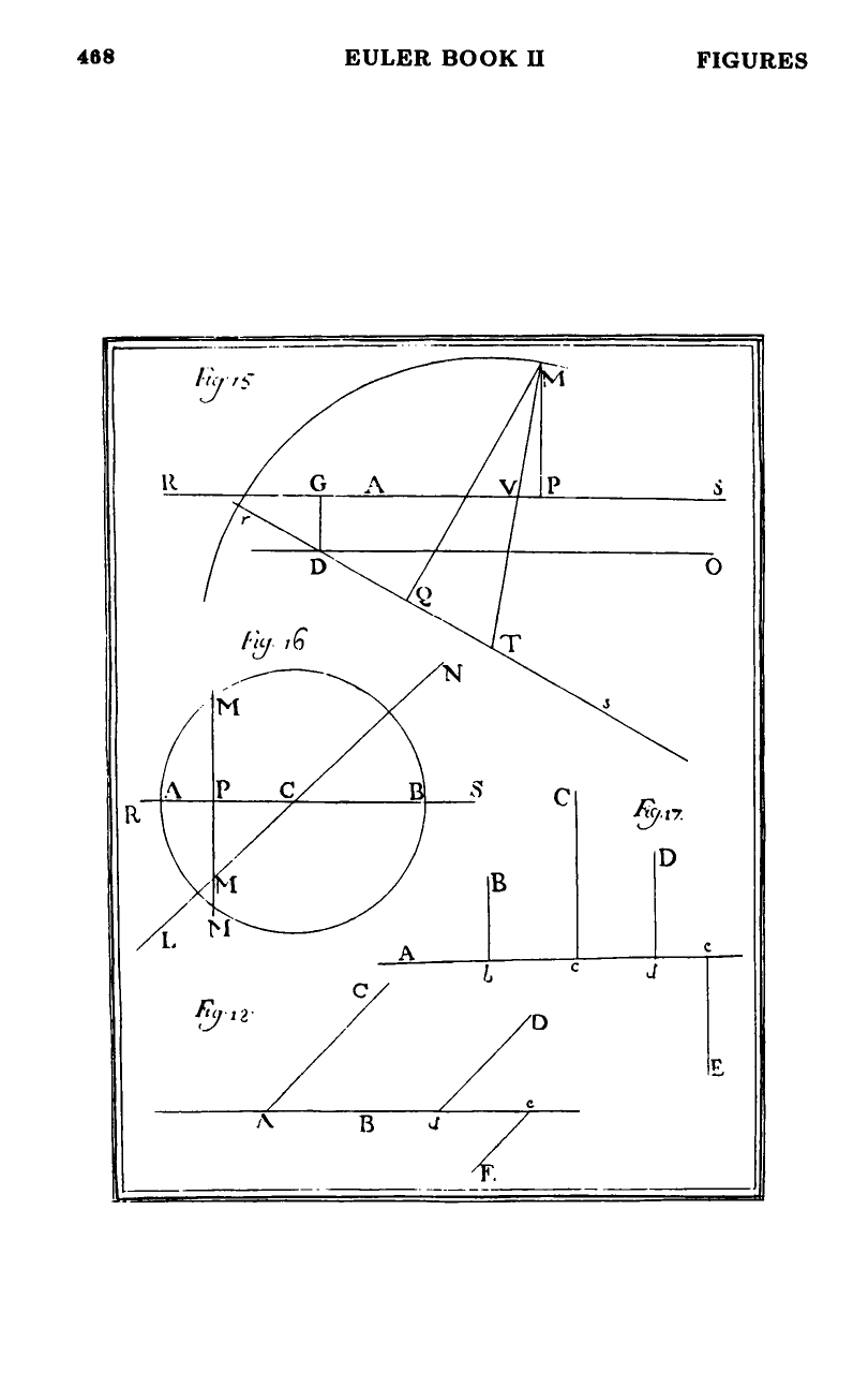
Figure 16: a circle with center $C$ and radius $CA=a$, together with a straight line $LN$ passing through $C$. Euler chooses the diameter $AB$ (with $AB$ at $45^{\circ }$ to $LN$) as the axis, origin at $A$, abscissa $AP=x$, ordinate $PM=y$.

Line equation. For a point on $LN$ with abscissa $AP=x$, geometry gives $PM=CP=a-x$, but $M$ lies below the axis, so $y=-(a-x)=x-a$, hence

$$y-x+a=0.$$

Circle equation. For a point on the circle, $P{M}^2=AP\cdot PB$ with $BP=2a-x$:

$$y^2=x(2a-x)⟺y^2+x^2-2ax=0.$$

Combined equation. Multiplying the two:

$$y^3-y^{2}x+y{x}^2-x^3+a{y}^2+3a{x}^2-2a^{2}x=0,$$

a third-degree equation that “contains both the straight line and the circle” (source: chapter3, §64).¹ Euler checks at $x=\frac{1}{2}a$: the cubic reduces to

$$y^3+\frac{1}{2}a{y}^2-\frac{3}{4}{a}^{2}y-\frac{3}{8}{a}^3=0,$$

which factors as $(y+\frac{1}{2}a)(y^2-\frac{3}{4}{a}^2)=0$, giving $y=-\frac{1}{2}a$ (the line) and $y=\pm \frac{1}{2}a\sqrt{3}$ (the circle) — three ordinates at one abscissa, exactly as the picture shows.

The counting lemma (§65)

A complex curve of order $n$ decomposes into simple curves whose orders sum to $n$. This is Euler’s version of “degrees multiply on product, so they add on factor”:

• Order 2 is either a simple conic, or complex = two straight lines.
• Order 3 is either a simple cubic, or straight line + conic, or three straight lines.
• Order 4 is either a simple quartic, or line + cubic, or two conics, or conic + two lines, or four lines.

The pattern extends to every higher order. In particular, curves of every lower order appear as components in every higher order — though only as complex curves, not as simple species (source: chapter3, §65).

Stated in one line: the partitions of $n$ enumerate the possible decomposition-types of complex curves of order $n$ into simple components (with each part matched to a species of that order).

Why the caveat matters for classification

The chapter’s central result — that order is determined by degree — tacitly assumes the curve is simple. Under reducibility the “order” reads as a sum rather than an intrinsic attribute of one curve:

• the equation $(y-x)(y-a)=0$ is of degree 2, but there is no degree-2 curve — only two degree-1 curves bundled together;
• so when general-equation-of-order-n reports $\frac{(n+1)(n+2)}{2}$ arbitrary constants at order $n$, a subset of those parameter choices lands in the reducible locus and does not yield a new species.

Enumerating the species at each order therefore requires restricting to irreducible equations. Complex curves are then handled trivially by reconstituting them from their simple components.

Forced reducibility: three collinear points on a “conic” (chapter 4, §79)

Chapter 4 gives a concrete way reducibility is forced by data: fit a conic through five points with three of them collinear. Because a simple conic meets a straight line in at most 2 points (line-curve-intersection-bound), no simple conic can contain the 3 collinear points; the unique order-2 equation through the 5 points therefore factors into two linear factors — the line through the 3 collinear points, and the line through the remaining 2. See curve-through-given-points for the construction.

Figures

Figures 15–18

Related pages

• chapter-3-on-the-classification-of-algebraic-curves-by-orders
• chapter-4-on-the-special-properties-of-lines-of-any-order
• line-curve-intersection-bound
• curve-through-given-points
• order-of-an-algebraic-curve
• general-equation-of-order-n
• continuous-and-discontinuous-curves
• straight-line-equation
• multi-valued-curves

Footnotes

1. The §64 cubic as printed appears to be missing a $-2axy$ term: expanding $(y-x+a)(y^2+x^2-2ax)$ directly gives $y^3-x{y}^2+x^{2}y-x^3+a{y}^2-2axy+3a{x}^2-2a^{2}x$. Euler’s reduced cubic at $x=\frac{1}{2}a$ does match the correct product (and the §64 check above uses it), so this looks like a printing slip in the source, not an error in the argument. ↩