Chapter 4: On the Special Properties of Lines of Any Order

Summary: Having defined the order of an algebraic curve in chapter 3, Euler now derives the first structural theorems about order. Three results anchor the chapter: (i) a line of order $n$ cannot intersect a straight line in more than $n$ points, proved by taking the straight line as axis and reading the polynomial in $x$ that results from $y=0$; (ii) the general equation of order $n$ has $\frac{(n+1)(n+2)}{2}$ arbitrary constants but only $\frac{n(n+3)}{2}$ independent determinations, because the equation is fixed only up to a common scalar; and (iii) an order-$n$ curve is therefore completely determined by $\frac{n(n+3)}{2}$ points — giving the sequence 2 (line), 5 (conic), 9 (cubic), 14 (quartic), 20 (quintic), …. The chapter closes with a detailed worked example: fitting a conic through five given points in oblique coordinates.

Sources: chapter4, figures15-18 (figures 17, 18)

Last updated: 2026-04-24

---

Why this chapter

chapter-3-on-the-classification-of-algebraic-curves-by-orders abstractly defined the order of a curve as the degree of its equation and showed (via degree-invariance) that order is coordinate-invariant. Chapter 4 converts that abstraction into two concrete handles. First, the intersection count with a straight line is bounded by the order — so order is directly visible geometrically, not only algebraically. Second, the data needed to specify an order-$n$ curve is a fixed finite number of points — so each order is parametrized by a concrete point-configuration problem. Together these make order operational: you can recognize one from a picture (partially — see §73) and you can construct one from data.

Structure of the chapter

§§66–72 — the intersection bound. line-curve-intersection-bound.

• §66: motivating claim. A straight line meets another straight line in one point; curves can meet a straight line in several. How many, at each order?
• §67: the method. In any equation for a curve, setting $y=0$ produces an equation in $x$ alone whose roots are the intersections with the axis.
• §68: bound on roots. The number of intersections is at most the highest power of $x$; if some roots are complex, it is strictly fewer.
• §69: order 1. $\alpha +\beta x+\gamma y=0$ with $y=0$ gives $\alpha +\beta x=0$, one intersection — or none, if $\beta =0$ (lines are parallel).
• §70: order 2. The general second-degree equation with $y=0$ leaves $\alpha +\beta x+\delta x^2$: two, one, or zero intersections. Never more than two.
• §71: order 3. Three intersections generically, possibly fewer if $\delta$ or other top coefficients vanish or roots are complex.
• §72: general $n$. A line of order $n$ cannot meet a straight line in more than $n$ points; equality is not forced, and there may even be no intersection.

§73 — the converse fails. From the number of intersections with a single straight line, the order cannot be inferred: $n$ intersections guarantee order $\ge n$, but the curve could be of higher order or even transcendental (see algebraic-and-transcendental-curves). “Whether it belongs to fourth order, or some higher order, or is transcendental we are unable to decide” (source: chapter4, §73).

§§74–75 — counting determinations. determinations-of-a-general-equation.

• §74: once the arbitrary constants in the general equation are fixed, the curve is fixed with respect to the given axis. Different values of the constants pick out different curves from the family.
• §75: but not every constant is independent. The first-degree equation $\alpha +\beta x+\gamma y=0$ has three constants but is determined by the ratios — divide through by any nonzero constant and only two determinations remain. Generalizing: the order-$n$ general equation has $\frac{(n+1)(n+2)}{2}$ constants but $\frac{(n+1)(n+2)}{2}-1=\frac{n(n+3)}{2}$ effective determinations.

§§76–81 — fitting a curve through points. curve-through-given-points.

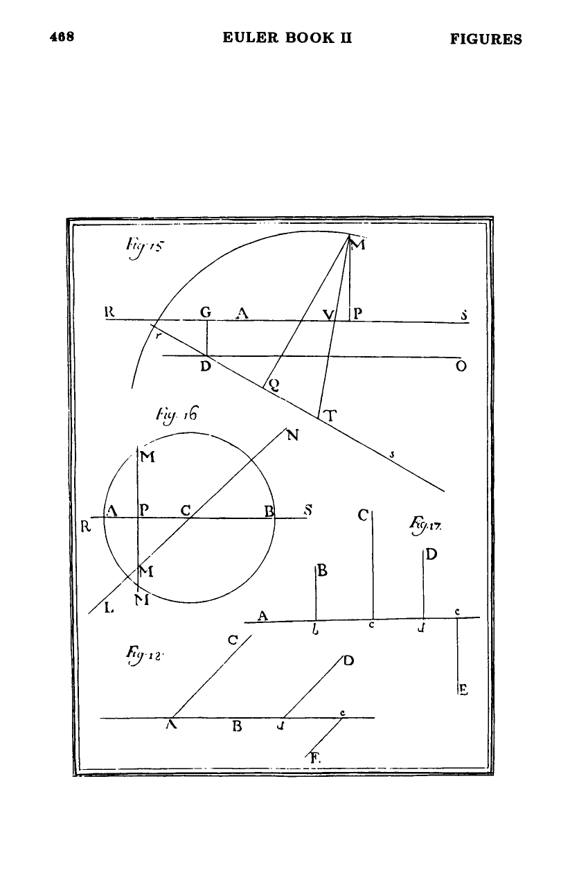
• §76 (figure 17): each point the curve must pass through yields one equation in the constants — drop a perpendicular from the point to the axis, and substitute the abscissa and ordinate into the general equation.
• §77: two points → two determinations used; three points → three; etc. As soon as the number of points equals the number of determinations, the curve is fixed.
• §78: order 1 needs 2 points — Euclid’s “two points determine a line”.
• §79: order 2 needs 5 points — the unique conic through five. Important caveat: if 3 of the 5 points are collinear, no continuous conic passes through all 5, because a conic cannot meet a straight line in 3 points (§70); the “solution” is then a complex curve, namely two straight lines (see complex-curves).
• §80: orders 3, 4, 5: 9, 14, 20 points respectively. In general, $\frac{n(n+3)}{2}$ points.
• §81: existence and uniqueness. Because the equations for the constants $\alpha ,\beta ,\gamma ,\dots$ are always linear, they can be solved without ever introducing quadratic or higher-degree extractions — so the coefficients are always real and single-valued. There is always a real curve through the prescribed points, and it is unique when the count is exactly right.

§§82–84 — practical technique and worked conic (figure 18).

• §82: pick the axis through one of the given points to kill $\alpha$; pick it through a second point so its ordinate is zero; use oblique coordinates so a third point lies on the ordinate direction. These choices reduce the system one equation at a time.
• §83 (figure 18): fit a conic through $A,B,C,D,E$. Take $A$ as origin, axis along $AB$, obliquity $\angle CAB$. With $AB=a$, $AC=b$, $Ad=c$, $Dd=d$, $Ae=e$, $eE=f$, the five points yield the linear system $\alpha =0,\gamma =-\zeta b,\beta =-\delta a,$ plus two further equations that collapse to $\delta =df(be-bc-de+cf),\zeta =ce(ad-af-de+cf).$ All coefficients are rational in the data, as §81 promised.
• §84: once the equation is determined, the curve is plotted by setting $x=0,1,2,3,\dots$ (and $-1,-2,\dots$) and solving the — at most quadratic in the conic case — equation for $y$.

Notable points

• The intersection bound unifies with chapter 3. Order was defined in chapter 3 as the degree of the equation; §§66–72 translate that into geometry — the degree equals the maximum number of times the curve can cross a straight line. The proof is just “set $y=0$ and count roots,” but the upshot is that from this chapter onward Euler can use intersection with a line as a diagnostic for order (from below), without opening up the equation.
• The §73 caveat is important. The bound $n\ge$ intersection-count goes one way only. A four-point intersection with a single straight line does not prove the curve is a quartic — it rules out quadratics and cubics, but the curve could be any higher order, or even transcendental. In modern terms: the generic line detects the order, but a single line only gives a lower bound.
• Why determinations count as $\frac{n(n+3)}{2}$ and not $\frac{(n+1)(n+2)}{2}$. The general equation is homogeneous in its constants — scaling every $\alpha ,\beta ,\gamma ,\dots$ by a common factor leaves the curve alone. So one degree of freedom is absorbed by the choice of “normalization.” Euler expresses this concretely in §75: in $\alpha +\beta x+\gamma y=0$, dividing through by $\alpha$ (if nonzero) leaves two free ratios $\beta /\alpha$ and $\gamma /\alpha$. The same reduction applies at every order.
• Why existence is never in doubt (§81). The usual worry with polynomial systems is that the solutions come out complex or multi-valued. Euler observes that here they do not: every equation in the constants, for every point, is linear in the constants. A linear system over the rationals has rational solutions (when determined). This is the reason the “fitting through points” story never degenerates into a classification of cases.
• The three-collinear-points exception (§79) is a bridge to chapter 3. It shows the intersection bound of §§66–72 and the complex-curves lemma of §65 working together: three points on a line cannot lie on any simple conic, so forcing five such points onto an order-2 equation produces the factored form $({\text{line}}_1)({\text{line}}_2)=0$ — a reducible curve. Classification and intersection theory are already interlocking.

What this buys for the rest of Book II

• A concrete programme for each order. Chapter 3 set up the “enumerate species at each order” problem. Chapter 4 puts a number on the size of that problem: order $n$ is a $\frac{n(n+3)}{2}$-parameter family, not a $\frac{(n+1)(n+2)}{2}$-parameter family. Species counts (e.g. the four conics at order 2, Newton’s cubic species at order 3) live in quotients of these parameter spaces.
• An existence theorem for conics and higher curves. §79’s “unique conic through 5 points” (modulo the three-collinear caveat) is the foundation on which later chapters analyze conics — every conic can be specified by, and constructed from, five points of it.
• A plotting algorithm (§84). Once the equation is pinned down, Euler will repeatedly use “substitute integer abscissas and solve for ordinates” as a practical way to draw the curve. This becomes the standard workflow for the remainder of Book II.

Figures

Figures 15–18

Related pages

• line-curve-intersection-bound
• determinations-of-a-general-equation
• curve-through-given-points
• chapter-3-on-the-classification-of-algebraic-curves-by-orders
• general-equation-of-order-n
• order-of-an-algebraic-curve
• complex-curves
• oblique-coordinates
• straight-line-equation