Oblique Coordinates

Summary: Coordinates in which the ordinate makes a fixed but not-necessarily-right angle with the axis. Every curve admits an equation in oblique coordinates for any chosen obliquity, axis, and origin, so the family of all oblique-plus-rectangular equations for a given curve is wider than the orthogonal family alone. Euler gives the substitutions for passing between rectangular and oblique systems, derives the most general equation of a curve (§45), and observes that the degree of the equation is still preserved (§46).

Sources: chapter2 (figures 14–15)

Last updated: 2026-04-24

---

Setup (§42)

Up through §41, Euler had always taken the ordinate perpendicular to the axis. The only change in this section is to relax that assumption: the ordinate $PM$ is drawn at a fixed angle $\varphi$ to the axis $RS$, not necessarily $90^{\circ }$. The pair $(x,y)=(AP,PM)$ is then a pair of oblique coordinates. The curve is the same; the description changes.

Since the axis, origin, and obliquity are each arbitrary, the family of equations for a given curve is now parametrized by five quantities: $f,g,m,n$ (the rigid motion parameters of coordinate-transformations) plus the obliquity angle. The rectangular case is the specialization $\varphi =90^{\circ }$.

Rectangular to oblique (§43)

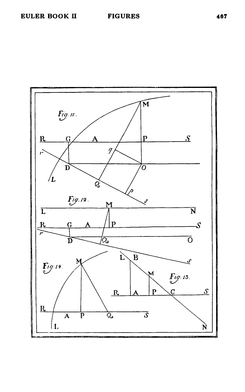
Keep the same axis $RS$ and origin $A$, but replace the orthogonal ordinate by the oblique one at angle $\varphi$. At a point $M$, let the orthogonal coordinates be $AP=x$, $PM=y$, and the oblique coordinates be $AQ=t$, $QM=u$ where $Q$ is the foot of the oblique ordinate and $M$ the same curve point (figure 14). Set $\sin \varphi =\mu$, $\cos \varphi =\nu$. In the right triangle $PMQ$,

$$\frac{y}{u}=\mu ,\frac{PQ}{u}=\frac{t-x}{u}=\nu .$$

Hence

$$u=\frac{y}{\mu },t=\nu u+x=\frac{\nu y}{\mu }+x,$$

and conversely

$$y=\mu u,x=t-\nu u.$$

Substituting $x=t-\nu u$ and $y=\mu u$ into a rectangular equation gives an oblique equation with obliquity $\varphi$.

Oblique to rectangular (§44)

Same figure, read backwards. Given an oblique equation in $t,u$ with obliquity $\varphi$, drop the perpendicular from $M$ to the axis to recover orthogonal coordinates $x=AP$, $y=PM$. Since

$$u=\frac{y}{\mu },t=\frac{\nu y}{\mu }+x,$$

substituting these for $u$ and $t$ in the oblique equation yields the rectangular equation.

The most general equation (§§45–46)

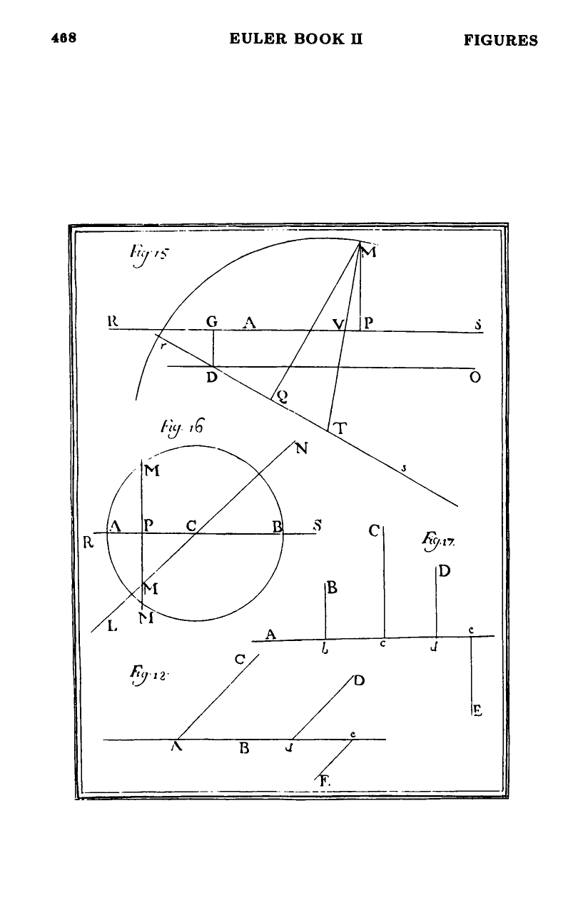
Combine the oblique substitution with the rigid motion of §§33–34. Start from a rectangular equation in $x,y$ for a curve $LM$. Choose any new axis $rs$ with any origin $D$ and any obliquity $\varphi$ (figure 15). Let $AG=f$, $DG=g$, and let the new axis make angle $q$ with the old (via $DO$ parallel to $RS$), with $\sin q=m$, $\cos q=n$. Let the new oblique coordinates be $DT=r$, $TM=s$, and the auxiliary rectangular-on-the-new-axis coordinates be $DQ=t$, $QM=u$. From §43 applied to the new axis,

$$t=r-\nu s,u=\mu s.$$

Combining with the rigid motion (§34), Euler arrives at

$$x=nr-(n\nu -m\mu )s-f,$$ $$y=-mr+(\mu n+\nu m)s-g.$$

He identifies $n\nu -m\mu =\cos (q+\varphi )$ as the cosine of the angle $AVM$ the new oblique ordinate makes with the old axis, and $\mu n+\nu m=\sin (q+\varphi )$ as its sine. Substituting these expressions for $x$ and $y$ into the original rectangular equation produces the most general equation of the curve — general in axis, origin, and obliquity alike (source: chapter2, §45).

Degree is still preserved (§46)

The substitutions above are still first-degree in $r,s$. Hence

the most general equation is of the same degree as the original equation in $x$ and $y$. It follows that no matter how the equation of a curve may be transformed by changing the axis and the origin and the inclination of the coordinates, still the equation keeps the same degree. (source: chapter2, §46)

Different degrees therefore remain a sure sign of different curves, even when the coordinate systems being compared are not both rectangular. See degree-invariance.

Figures

Figures 11–14

Figures 15–18

Related pages

• chapter-2-on-the-change-of-coordinates
• coordinate-transformations
• general-equation-of-a-curve
• degree-invariance
• straight-line-equation
• abscissa-and-ordinate