curve-through-given-points

Fitting a Curve of Order $n$ Through Given Points

Summary: An algebraic curve of order $n$ is completely determined by $\frac{n(n+3)}{2}$ points through which it is required to pass — giving the sequence 2, 5, 9, 14, 20, 27, … for orders $n=1,2,3,4,5,6,\dots$. Each point yields one linear equation in the constants of the general equation. Because the system is linear, the coefficients of the fitted curve are always real and uniquely determined (§81). When fewer points are prescribed, an infinite family remains; when the count is exactly $\frac{n(n+3)}{2}$, the curve is unique, with one important exception — configurations that would force a simple curve to violate the line-curve-intersection-bound instead yield a reducible equation.

Sources: chapter4, figures15-18 (figures 17, 18)

Last updated: 2026-04-24

---

The basic procedure (§§76–77, figure 17)

We can always define the arbitrary constants in such a way that the curve will pass through a given point. This gives rise to one of the determinations. (source: chapter4, §76)

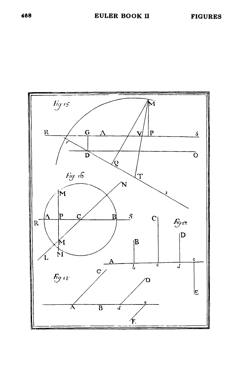
Given the general equation of order $n$ and a point $B$ through which the curve must pass (figure 17): choose any axis with origin $A$, drop the perpendicular $Bb$ from $B$ to the axis, and read off the abscissa $Ab$ and ordinate $Bb$. Substituting these values into the general equation yields a linear equation in the constants $\alpha ,\beta ,\gamma ,\delta ,\dots$. This equation pins down one of them in terms of the others — one determination used.

A second point $C$ gives a second linear equation (§77); $k$ points give $k$ linear equations. As long as $k$ is at most the number of determinations $\frac{n(n+3)}{2}$, the system has solutions; when $k$ equals that count, the solution is (generically) unique.

Order by order (§§78–80)

Order 1: two points (§78). The general first-degree equation has 2 determinations; two given points uniquely specify a straight line. This recovers Euclid’s Elements I.Postulate 1 — “a straight line may be drawn from any point to any other point” — from the algebraic side. With fewer than 2 points the line is underdetermined (infinitely many lines through one point).

Order 2: five points (§79). The general second-degree equation has 5 determinations; five given points uniquely specify a conic section. Four or fewer points leave an infinite family of conics. See the caveat below.

Order 3: nine points (§80). The cubic has 9 determinations — the “unique cubic through 9 points” fact. Historically the starting point of Newton’s classification of cubics.

Order 4: fourteen points (§80). 14 points fix a quartic.

Order 5: twenty points (§80). 20 points fix a quintic.

Order $n$: $\frac{n(n+3)}{2}$ points. Euler states the formula in §80–81. The sequence for $n=1,2,3,4,5,6,7,\dots$ is $2,5,9,14,20,27,35,\dots$

Existence and uniqueness (§81)

Unless more than $\frac{n(n+3)}{2}$ points are proposed, there is always one or an infinite number of lines of order $n$ which pass through these points. There will be exactly one line if the number of points is $\frac{n(n+3)}{2}$, and an infinite number if there are fewer points. It will never happen, no matter how the points may be placed, that the solution cannot be found. (source: chapter4, §81)

Two facts worth separating:

1. The solution is always real. The determining equations in the constants are linear (a point substituted into the general equation gives a linear relation between $\alpha ,\beta ,\dots$). A linear system with rational coefficients has rational solutions — never imaginary, never multi-valued, never requiring a quadratic or higher extraction. So the fitted curve’s coefficients are automatically real.
2. The solution is generically unique. With exactly $\frac{n(n+3)}{2}$ points and the system nondegenerate, exactly one curve. With fewer points, infinitely many.

Euler is emphatic: “It will never happen, no matter how the points may be placed, that the solution cannot be found.” This is stronger than mere existence — it promises that the real solution is always available, not hidden behind complex roots. The source of this promise is the linearity of the system, which in turn is the reason the counting argument of §75 works cleanly.

The three-collinear-points exception (§79)

If three of the five points lie on a straight line, then, since a second order line cannot intersect a straight line in three points, there is no continuous curve which will pass through those points. Rather we will have a complex line, that is, two straight lines. (source: chapter4, §79)

This is the one subtlety in the existence claim. Because a simple conic meets any straight line in at most 2 points (line-curve-intersection-bound, §70), three of the five given points cannot be collinear if the fitted conic is to be simple. If they are, the unique order-2 equation through the five points factors as a product of two linear factors — that is, it is a complex curve: the line through the three collinear points, together with a second line through the other two.

This is not a failure of the §81 existence theorem, but a reminder that the theorem produces some curve of order $n$, which may turn out to be reducible. The “unique conic through 5 points” statement is tacitly “unique simple conic, provided no 3 points are collinear.”

The analogous exceptions arise at higher orders. For an order-$n$ curve, any subconfiguration of $k$ points lying on a curve of order $m<n$ where $k>m\cdot n$ (the intersection-bound max) forces reducibility; see complex-curves for the order-decomposition lemma.

Practical technique (§§82–83, figure 18)

The linear system simplifies dramatically if the axis is placed through some of the given points.

Axis through one point (§82). Make the first point $A$ the origin. Then its abscissa and ordinate are both zero, and substituting into the general equation yields $\alpha =0$. The constant term disappears immediately.

Axis through a second point. Make the axis pass through point $B$ so $B$‘s ordinate is zero. Substituting $x=AB$, $y=0$ gives an equation containing only the constants on $x^j$.

Oblique coordinates. Let a third point $C$ sit directly above $A$ along the ordinate direction: the angle $\angle CAB$ is then the obliquity of the coordinate system (see oblique-coordinates). At $C$, $x=0$, so substituting gives an equation in the constants on $y^j$.

Worked conic example (§83, figure 18). Fit a conic through five points $A,B,C,D,E$. Take $A$ as origin; axis along $AB$; $\angle CAB$ as the obliquity. Drop ordinates $Dd,Ee$ from $D,E$ parallel to $AC$. Let

$$AB=a,AC=b,Ad=c,Dd=d,Ae=e,eE=f.$$

The five coordinates are $(0,0),(a,0),(0,b),(c,d),(e,f)$. Substituting into the general conic equation

$$\alpha +\beta x+\gamma y+\delta x^2+ϵxy+\zeta y^2=0$$

gives the five linear equations (source: chapter4, §83):

$$\begin{array}{rl}\text{I.}& 0=\alpha \\ \text{II.}& 0=\alpha +\gamma b+\zeta b^2\\ \text{III.}& 0=\alpha +\beta a+\delta a^2\\ \text{IV.}& 0=\alpha +\beta c+\gamma d+\delta c^2+ϵcd+\zeta d^2\\ \text{V.}& 0=\alpha +\beta e+\gamma f+\delta e^2+ϵef+\zeta f^2\end{array}$$

Equations I–III are solved on sight: $\alpha =0,\gamma =-\zeta b,\beta =-\delta a.$

Substituting into IV and V:

$$\begin{array}{rl}0& =-\delta ac-\zeta bd+\delta c^2+ϵcd+\zeta d^2\\ 0& =-\delta ae-\zeta bf+\delta e^2+ϵef+\zeta f^2\end{array}$$

Multiply the first by $ef$, the second by $cd$, subtract to eliminate $ϵ$:

$$0=\delta \cdot ce(ad-af-de+cf)+\zeta \cdot df(bc-be+de-cf).$$

Rewriting as a ratio:

$$\frac{\delta }{\zeta }=\frac{df(be-bc-de+cf)}{ce(ad-af-de+cf)}$$

so that (up to the common scaling discussed in determinations-of-a-general-equation):

$$\delta =df(be-bc-de+cf),\zeta =ce(ad-af-de+cf).$$

One remaining equation then gives $ϵ$. All coefficients are polynomial expressions in the data, as §81 guaranteed — no square roots, no case splits. (source: chapter4, §83)

Plotting the fitted curve (§84)

Once the equation is determined, the curve is drawn point by point: assign the abscissa $x$ successive integer values $0,1,2,3,\dots$ and $-1,-2,-3,\dots$, and solve the equation for the corresponding ordinate(s) $y$. At order 2 the equation is quadratic in $y$ and yields at most two ordinates per abscissa; at order $n$, at most $n$ ordinates per abscissa. “In this way we obtain many points of the curve which are sufficiently close together” (source: chapter4, §84).

This is Euler’s practical prescription for making a picture from an equation. It is the workflow he will use repeatedly in later chapters when discussing specific curves.

Why linear, not polynomial

The remarkable feature of the point-fitting problem is that every equation in the constants is linear, no matter how high the order of the curve. This is because the general equation is linear in its constants (even though it is high-degree in $x,y$): each monomial $x^i{y}^j$ sits next to exactly one constant. Substituting specific values for $x,y$ just evaluates the monomials, leaving a linear expression in the constants. So no matter how exotic the curve Euler wants to fit, the arithmetic stays linear.

This is the algebraic reason behind §81’s existence-and-uniqueness promise — and why the dimension count of determinations-of-a-general-equation exactly tracks the number of points needed.

Figures

Figures 15–18

Related pages

• chapter-4-on-the-special-properties-of-lines-of-any-order
• determinations-of-a-general-equation
• general-equation-of-order-n
• line-curve-intersection-bound
• complex-curves
• straight-line-equation
• oblique-coordinates
• order-of-an-algebraic-curve