Chapter 5: On Second Order Lines

Summary: Euler devotes a full chapter to the second-order lines — the conic sections — because they are the simplest curves and “have the widest application throughout the whole of the more sophisticated geometry” (source: chapter5, §85). Working from the general equation $\alpha +\beta x+\gamma y+\delta x^2+ϵxy+\zeta y^2=0$ rewritten as a quadratic in $y$, Euler derives a long list of metric and projective properties without any reference to the cone: every conic has a diameter that bisects parallel chords; rectangles on parallel chords are in fixed ratio (chord-rectangle-property); all diameters meet in a single point — the center — that bisects each of them; every diameter has a conjugate and the sum of squares of any conjugate pair is constant; tangents at the ends of any diameter together with a third tangent generate Newton’s tangent ratios $AK\cdot BL=C{E}^2$; and there is exactly one orthogonal pair — the principal axes — leading to the focal-polar equation and the latus rectum machinery used by all later treatments.

Sources: chapter5, figures19-22, figures23-25, figures26-29, figures30-32

Last updated: 2026-04-25

---

Why this chapter

chapter-3-on-the-classification-of-algebraic-curves-by-orders already showed that every order-2 curve fits the six-coefficient equation, and chapter-4-on-the-special-properties-of-lines-of-any-order showed that any 5 points (not three of them collinear) determine such a curve uniquely. Chapter 5 is the inevitable next step: extract from that one equation everything geometric that conics have in common, before breaking them into species (parabola, ellipse, hyperbola — that comes in chapter 6). Euler’s stance is explicit: “We will investigate here only those properties which flow directly from the equation” (source: chapter5, §85). No cone, no synthetic case-splitting — just algebraic manipulation of the quadratic-in-$y$ form, with two roots whose sum and product encode the geometry.

Two algebraic facts drive the entire chapter. From $y^2+\frac{ϵx+\gamma }{\zeta }y+\frac{\delta x^2+\beta x+\alpha }{\zeta }=0$ the sum of roots $PM+PN=-\frac{ϵx+\gamma }{\zeta }$ gives the diameter property (§§87–92), and the product of roots $PM\cdot PN=\frac{\delta x^2+\beta x+\alpha }{\zeta }$ gives the rectangle ratios (§§92–100). Everything else — center, conjugate diameters, tangent rectangles, foci — is built on these two.

Structure of the chapter

§§85–86 — set-up. The general equation, rewritten as a quadratic in $y$. Each abscissa $x$ has either two ordinates (real roots), one (a double root, tangent), or none (complex). The case $\zeta =0$ is benign — one ordinate has receded to infinity.

§§87–91 — diameters from the sum of roots. diameter-of-conic.

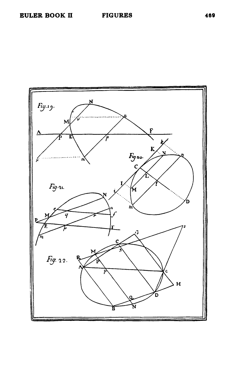
• §87 (figure 19): if both ordinates $PM,PN$ are real, $PM+PN=-(ϵx+\gamma )/\zeta$. Comparing two parallel ordinates $PMN$ and $pmn$ yields $M\mu +N\nu =ϵPp/\zeta$ — the difference of midpoint heights is a fixed multiple of the difference of abscissas, no matter where the chords are drawn.
• §88 (figure 20): tangent at a point of contact $C$, plus a “chord ordinate” $KCI$ parallel to the chosen chord direction. Ratio $\frac{MI}{mi}=\frac{CI-CK}{Ci-Ck}$.
• §89: pick $MI$ so $CI=CK$ — the tangent-parallel through the chord midpoint. Then $MI/mi=0$, so all parallel chords are bisected by the same line $CL\ell$.
• §90: that line $CL\ell$ is called the diameter. Every conic has innumerably many diameters: one per direction of chord.
• §91: dual construction — pick any two parallel chords, bisect them, and the line through the two midpoints is a diameter. Where the diameter meets the curve, the tangent there is parallel to the bisected chords.

§§92–100 — rectangles from the product of roots. chord-rectangle-property.

• §92 (figure 19): $PM\cdot PN=(\delta x^2+\beta x+\alpha )/\zeta$. If the axis cuts the curve at $E$ and $F$, this factors as $\frac{\delta }{\zeta }(x-AE)(x-AF)=\frac{\delta }{\zeta }PE\cdot PF$.
• §93 (figure 21): hence $\frac{PM\cdot PN}{PE\cdot PF}=\frac{\delta }{\zeta }$, a constant. The same ratio holds for any pair of transverse chord-systems: $\frac{PM\cdot PN}{PE\cdot PF}=\frac{qM\cdot qN}{qe\cdot qf}$ — the second general property.
• §94 (figure 24): when $M,N$ coincide the chord becomes tangent and $PM\cdot PN\to P{C}^2$. Hence $\frac{P{C}^2}{PM\cdot PN}=\frac{p{C}^2}{pm\cdot pn}$ — the tangent-rectangle ratio.
• §95 (figure 20): along a diameter as axis, with half-chord $LM=y$, $LD=a-x$, the equation collapses to $y^2=\frac{h}{k}(ax-x^2)$ — the diameter-form equation of the conic.
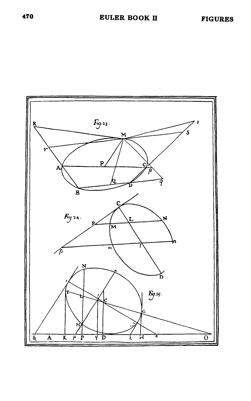
• §96–98 (figure 22): inscribed quadrilateral $ACDB$ with parallel sides $AB,CD$. Through any other point $M$ of the curve draw $MQ\parallel AB$ and $MS\parallel BD$. Then $\frac{MP\cdot MQ}{MR\cdot MS}$ is constant.
• §99 (figure 23): generalization to the inscribed trapezium $ABCD$. From any point $M$ on the curve, drop $MP,MQ,MR,MS$ to the four sides at fixed angles. Then $\frac{MP\cdot MQ}{MR\cdot MS}$ is fixed — the projective form of the conic property.
• §100 (figure 24): geometric mean construction. If $L$ on chord $MN$ satisfies $P{L}^2=PM\cdot PN$, the line through $C$ (point of contact of the tangent) and $L$ cuts every parallel chord in its geometric mean.

§§101–108 — the center. center-of-conic.

• §101 (figure 25): the diameter for ordinates of slope $ϵ/\zeta$ has equation $2\zeta z+ϵx+\gamma =0$.
• §102: length of that diameter from $(AK-AH{)}^2$, using the sum and product of roots of $z^2$-equation $z^2-\frac{2(\beta \zeta -ϵ\gamma )}{{ϵ}^2-4\delta \zeta }z+\frac{{\gamma }^2-4\alpha \zeta }{{ϵ}^2-4\delta \zeta }=0$. Crucially $I{G}^2$ depends only on coefficients, not on the obliquity.
• §103–105: under an oblique coordinate change with sine $\mu$, cosine $\nu$, the diameter equation transforms to $(2{\mu }^2\zeta +\mu \nu ϵ)q+(\mu ϵ+2\nu \delta )p+\mu \gamma +\nu \beta =0$.
• §106: the intersection $C$ of two diameters $IG$ and $ig$ is computed from the two diameter equations. The result has $\mu ,\nu$ cancelling: the intersection is the same point regardless of obliquity. Coordinates of $C$: $AD=g=\frac{2\beta \zeta -\gamma ϵ}{{ϵ}^2-4\delta \zeta },CD=h=\frac{2\gamma \delta -\beta ϵ}{{ϵ}^2-4\delta \zeta }.$
• §107: all diameters pass through this point — and any chord through it is a diameter. Euler names this point the center.
• §108: the center is the midpoint of every diameter.

§§109–115 — center as origin; conjugate diameters. conjugate-diameters.

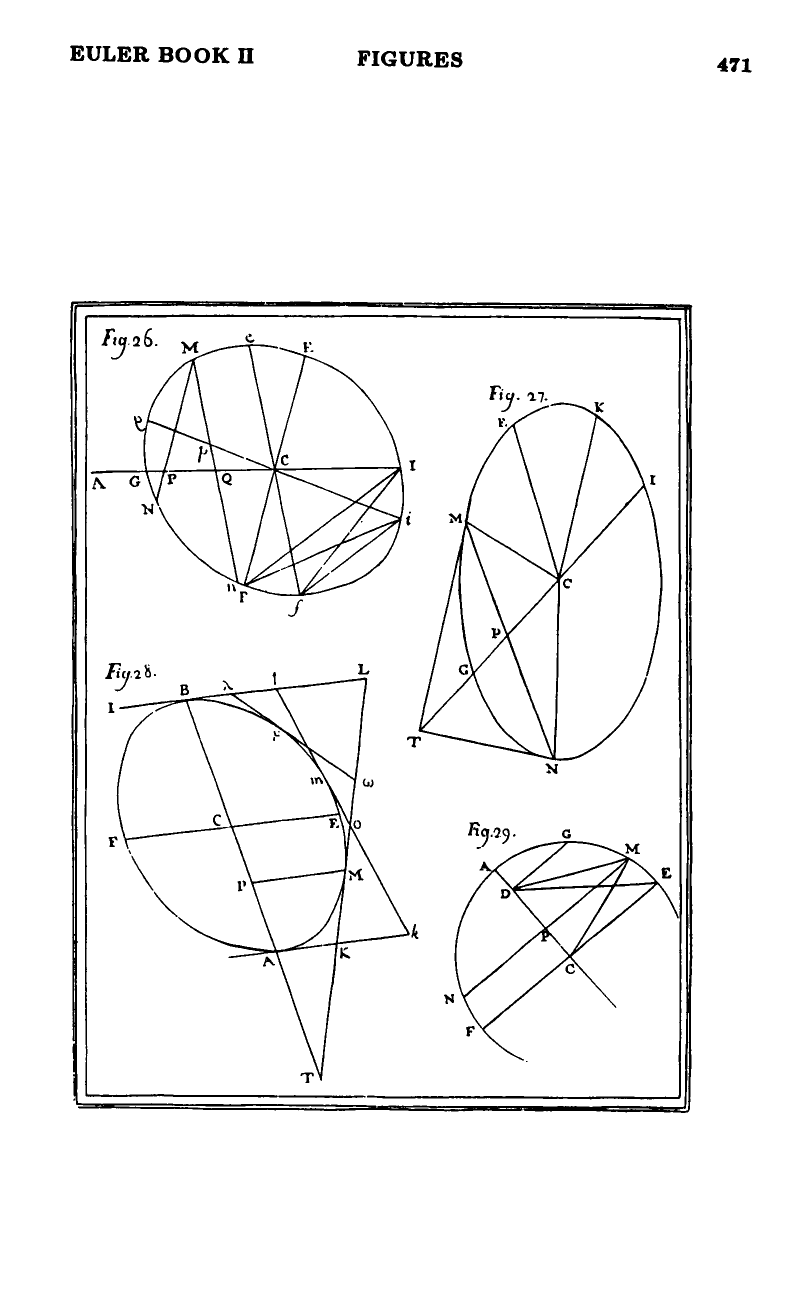
• §109–110 (figure 26): take any diameter as axis, place the origin at the center. The general equation reduces to $y^2=\alpha -\beta x^2$. Diameter length $GI=2\sqrt{\alpha /\beta }$.
• §111: setting $z=0$ gives the chord through the center parallel to the ordinates: $CE=CF=\sqrt{\alpha }$. The chord $EF$ is itself a diameter, and bisects all chords parallel to $GI$. Each of the two diameters $GI,EF$ bisects all chords parallel to the other — they are conjugate (Euler’s term, §111).
• §112–115: under an oblique change of axes, the conjugate-pair structure is preserved. Semidiameters in the new direction satisfy $a=f\sqrt{\frac{\sin q\sin (q+\pi )}{\sin (q-p)\sin (q+\pi -p)}},b=g\sqrt{\frac{\sin q\sin (q-p)}{\sin (q+\pi )\sin (q+\pi -p)}}$ where $f,g$ are the original conjugate semidiameters.
• §116–117: $ab\sin (q+\pi -p)=fg\sin q$ — the parallelograms inscribed around any conjugate pair are equal in area.
• §118–120 (figure 27): tangent at any point $M$ is constructed via the conjugate semidiameter $CK$ to the semidiameter $CM$. From this, $C{E}^2+C{G}^2=C{K}^2+C{M}^2$: the sum of squares of any pair of conjugate semidiameters is constant.

§§121–124 — tangent properties (Newton’s Principia lemmas). tangent-properties-conic.

• §121–122 (figure 28): tangents $AK,BL$ at the ends of a diameter $AB$, and a third tangent $MT$ at any point $M$, with $K,L$ the intersections of $MT$ with the other two tangents. Then $AK\cdot BL=C{E}^2$ — the constant rectangle of tangent intercepts.
• §123: extend to a fourth tangent: with intersection $o$ of $KL$ and $kl$, $\frac{Ko}{Lo}=\frac{AK}{Bl}$, etc.
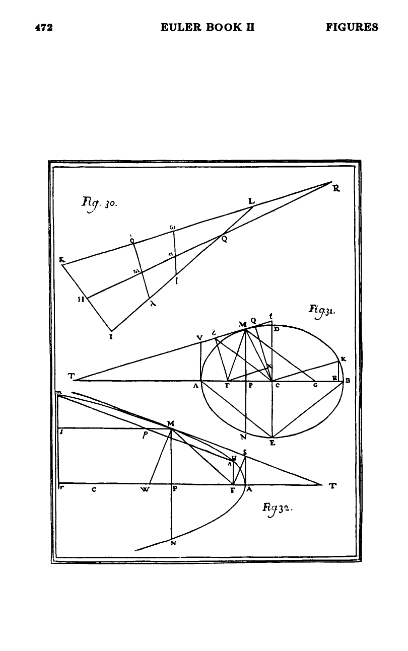
• §124 (figure 30): three tangents form a triangle in which any transversal cuts the two paired sides in the same ratio.

§§125–130 — principal axes, focus, latus rectum. principal-axes-and-foci.

• §125 (figure 27): among all conjugate pairs, exactly one is orthogonal. Solving $\cot 2q+\frac{C{G}^2}{C{E}^2\sin 2q}=0$ for $q$ gives the angle of that pair.
• §126–127 (figure 29): take that orthogonal pair as the principal axes. Equation: $y^2=b^2-\frac{b^2}{a^2}{x}^2$. When $a=b$ all radii are equal — circle.
• §128: there are two points $D$ on the principal axis at distance $\sqrt{a^2-b^2}$ from the center such that any straight line $DM$ from $D$ to the curve has rational length in $x$.
• §129: these are the foci (or navels). The principal axis is the transverse axis, the orthogonal one the conjugate axis. The ordinate at the focus, $DG=b^2/a$, is the semilatus rectum; doubled, the latus rectum (parameter). The endpoints of the transverse axis are the vertices; the tangent at a vertex is perpendicular to the principal axis.
• §130: focal polar equation. With focus–vertex distance $d$ and semilatus rectum $c$, the focal radius at angle $v$ from the principal axis is $DM=\frac{cd}{d-(d-c)\cos v}.$

Notable points

• Algebra without the cone. Apollonius derived conic properties from sections of a cone; Euler refuses. Every theorem here comes from the quadratic-in-$y$ form alone — sum and product of roots, comparison of two chords, substitution of coordinate transforms. The chapter is a demonstration that analytic geometry can recover all the classical conic properties without invoking the cone or any synthetic case-split into ellipse/parabola/hyperbola. (The case-split is deferred to chapter 6.)
• Two algebraic facts, two strands of geometry. Sum of roots → diameters and bisection; product of roots → rectangles, tangent constructions, and ultimately foci. Every result in §§87–130 is a downstream consequence of one of these.
• The center is intrinsic (§106). Although the diameter equations depend on obliquity $\mu ,\nu$, their intersection — the center — does not. Euler’s calculation in §106 makes the cancellation explicit: $\mu$ and $\nu$ drop out. This is a coordinate-invariance statement of the same flavor as degree-invariance.
• Conjugate diameters generalize the principal axes. With the equation $y^2=\alpha -\beta x^2$ in any diameter-aligned, center-origin frame, the role of “axis” and “perpendicular axis” can be played by any conjugate pair, not just the orthogonal one. The orthogonal pair (§125) is special because it always exists and is unique, but it is one choice among infinitely many for the same conic.
• $AK\cdot BL=C{E}^2$ is the lever for Newton. §122 is the projective property Newton invokes throughout the Principia to derive Kepler’s laws — which Euler explicitly notes (“These are the main properties of conic sections from which NEWTON found the solution to many important problems in his Principia”, source: chapter5, §122).
• Foci appear as a rationality miracle (§128). Euler does not introduce foci by their distance-sum/distance-difference characterization; he introduces them as the unique points $D$ on the principal axis from which $DM$ is a rational function of $x$. The classical metric description follows. The subordination of the metric to the algebraic is characteristic of his style.
• The focal polar equation (§130) is the bridge to dynamics. $DM=\frac{cd}{d-(d-c)\cos v}$ is the form Newton’s gravitational analysis uses — orbits as conics with the gravitating body at a focus. By the end of the chapter Euler has the equation in hand, though chapters 6–7 will untangle the case-split into ellipses, parabolas, and hyperbolas.

What this buys for the rest of Book II

• Chapter 6 specializes to the case-split (parabola if ${ϵ}^2-4\delta \zeta =0$; ellipse if $<0$; hyperbola if $>0$) — using the same general equation but now reading off the species from the discriminant.
• Chapters 7–9 investigate parabolas, ellipses, and hyperbolas individually, with the focal polar equation of §130 as starting point.
• The diameter/center/conjugate/tangent machinery developed here transfers directly: every theorem is stated for “second-order lines” in general and applies unchanged to all three species.

Figures

Figures 19–22

Figures 23–25

Figures 26–29

Figures 30–32

Related pages

• diameter-of-conic
• chord-rectangle-property
• center-of-conic
• conjugate-diameters
• tangent-properties-conic
• principal-axes-and-foci
• chapter-3-on-the-classification-of-algebraic-curves-by-orders
• chapter-4-on-the-special-properties-of-lines-of-any-order
• general-equation-of-order-n
• oblique-coordinates
• coordinate-transformations