Intersection of Two Curves

Summary: To find the intersections of two curves expressed by equations in the common coordinates $(z,y)$, eliminate $y$ to obtain a polynomial in $z$ alone; its real roots give the abscissas of the intersections, and the corresponding ordinates are read off from either original equation. The same procedure underlies the line-curve intersection bound of line-curve-intersection-bound, but generalizes to two arbitrary algebraic curves.

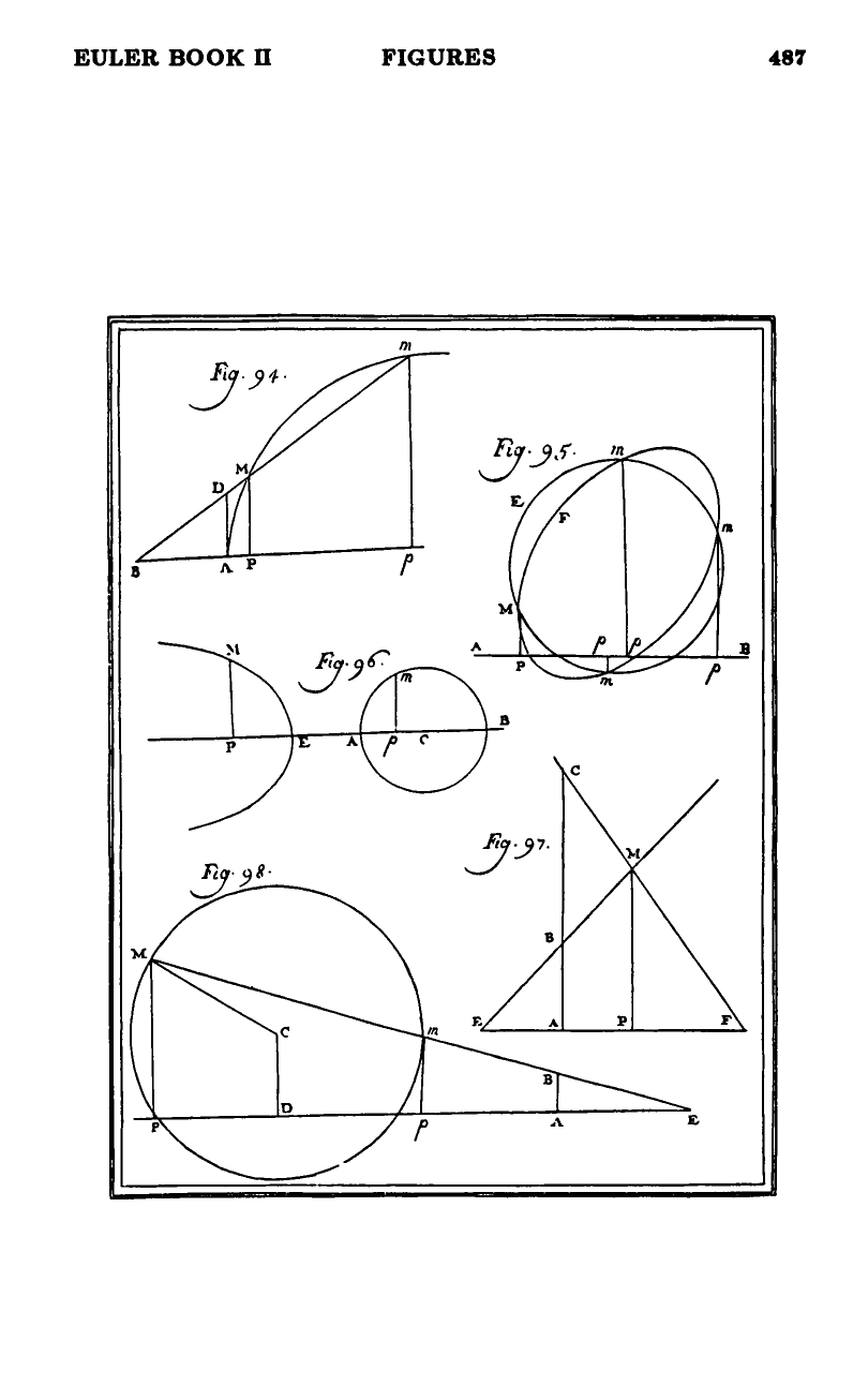
Sources: chapter19 (§§457–464), figures94-98 (figures 94, 95).

Last updated: 2026-05-12.

---

The procedure (§§457–464)

Let two curves be given by

$F(z,y)=0,G(z,y)=0$

in the same rectangular coordinates with the same origin and axis. At an intersection point, the values of $z$ and $y$ satisfy both equations simultaneously.

1. Eliminate $y$: combine the two equations to produce a single equation $R(z)=0$ containing only $z$ and known constants.
2. Solve for $z$: the real roots of $R(z)=0$ are the abscissas $AP,Ap,A{p}^{\prime },\dots$ of the candidate intersection points.
3. Recover $y$: substitute each root back into either original equation to obtain the corresponding ordinate $PM,pm,\dots$.

When one curve is a straight line $\alpha z+\beta y=\gamma$, the substitution $y=(\gamma -\alpha z)/\beta$ into the equation of the curve is immediate and reduces $y$ to a single-valued function of $z$. Every real root of the resulting polynomial then corresponds to a true intersection. This is the classical line-curve case (line-curve-intersection-bound).

For two genuine curves (figure 95), the elimination is more delicate: each curve can be a multi-valued function of $z$, and the resulting equation in $z$ may admit roots whose corresponding ordinate values are complex — a phenomenon Euler isolates as the complex intersection (complex-intersections).

Why eliminate $y$ rather than just intersect ordinates (§461)

Once the abscissas $AP,Ap,\dots$ are known, one could erect the ordinates and look for points where they meet either curve. But each ordinate can intersect a curve at several heights, so it is unclear which of those heights is the actual intersection. Eliminating $y$ instead delivers the ordinate value directly at each abscissa, without consulting either curve a second time.

When two of the roots $z$ coincide, the two intersection points $M$ and $m$ merge into one. This is either a tangency or a double point of the multi-point type — distinguished by whether the merged point is a smooth tangent contact or a transverse self-crossing.

Number of intersections (§§460, 462)

The substitution $y=(\gamma -\alpha z)/\beta$ from a linear equation enters $y$ only to the first power, so the substituted polynomial has the same degree as the original curve equation in $z$ and $y$ (or lower if the leading $z$-coefficient drops out under summation). Hence:

• The number of intersections of a curve of order $n$ with a straight line is at most $n$, recovering line-curve-intersection-bound as a corollary.
• More generally, the number of real intersections of two curves is at most the degree of the eliminant in $z$ — a bound which, in modern terms, equals $mn$ for curves of orders $m$ and $n$ (Bézout’s theorem). Euler hints at this in §457 but the explicit $mn$ statement is deferred to chapter 20.

If the eliminant has no real roots, the curves do not meet and the straight line is not even tangent. If it has real roots whose corresponding ordinates are complex, there are complex intersections but no real ones — see complex-intersections.

Worked example: parabola vs. circle (§465)

Take the parabola $y^2-2zy+z^2-2az=0$ and the circle $y^2+z^2-c^2=0$. Subtracting,

$2zy+2az-c^2=0⟹y=\frac{c^2-2az}{2z},$

so $y$ is a non-irrational (single-valued rational) function of $z$. Substituting into the circle’s equation,

$c^4-4a{c}^{2}z+4(a^2-c^2)z^2+4z^4=0.$

Each real root of this quartic in $z$ corresponds to a true intersection. With $c=2a$ the quartic becomes $4a^4-4a^{3}z-3a^2{z}^2+z^4=0$, factoring as $(z-2a)(z^3+2a{z}^2+a^{2}z-2a^3)=0$; the root $z=2a$ gives $y=0$, i.e., an intersection on the axis.

Because $y$ here is a single-valued function of $z$, this example escapes complex intersections entirely.

Figures

Figures 94–98

Related pages

• line-curve-intersection-bound
• complex-intersections
• elimination-of-ordinate
• indeterminate-multiplier-elimination
• chapter-19-on-the-intersection-of-curves
• multiple-points-on-curves