Chapter 20 — On the Construction of Equations

Summary: Chapter 20 inverts chapter 19. Where chapter 19 takes two given curves and reads off the polynomial whose roots are the abscissas of their intersection points, chapter 20 takes a given polynomial $\Phi (z)=0$ and asks for two curves whose intersections realize its roots as visible line segments. The chapter develops four sample constructions — line + line for a linear equation (§488); line + circle for a quadratic (§§489–491), and two circles as an alternative (§492); circle + parabola for a biquadratic, with the cubic as a limiting case (§§493–495) — and then a general method using a single-valued first curve $P+Qy=0$ to construct any equation of any degree (§§499–504). The intersection-degree bound $mn$ (§§496–498) governs how to factor the target degree into orders of two construction curves.

Sources: chapter20 (§§486–505); figures 97, 98 in figures94-98; figures 99, 100 in figures99-102.

Last updated: 2026-05-12.

---

The chapter at a glance

Chapter 19’s elimination procedure takes two equations $F(z,y)=0$ and $G(z,y)=0$ and produces a polynomial $\Phi (z)=0$ whose real roots locate the real intersection abscissas. Chapter 20 reverses the arrow: given $\Phi (z)=0$, find $F$ and $G$. The chapter divides into three movements:

1. Constructions for low degrees (§§486–495). Sample constructions for the linear, quadratic, and biquadratic equations using the simplest possible curve pairs.
2. The general degree bound (§§496–498). Two curves of orders $m$ and $n$ meet in at most $mn$ points; the bound dictates how to factor a target degree.
3. The general construction method (§§499–505). For any equation of any degree, choose the first curve in the form $P(z)+Q(z)y=0$ (so $y$ is single-valued in $z$ and no complex intersections are possible), then solve for the second curve by substitution.

See construction-of-equations for the master concept and intersection-product-degree-bound for the joint-degree count.

1. Low-degree constructions (§§486–495)

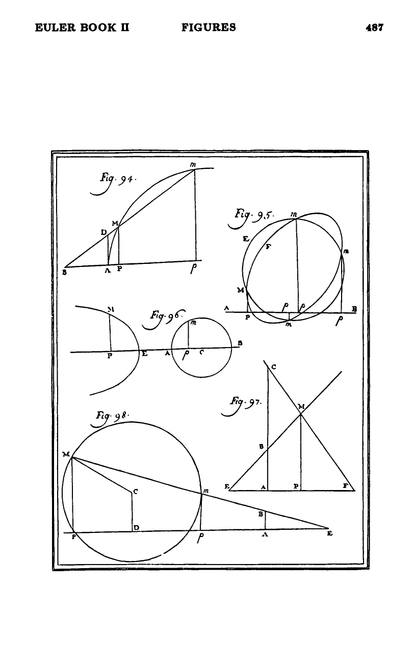
Linear by two lines (§488, figure 97)

Two lines crossing at $M$; algebra gives $z=ab(d-c)/(bc+ad)$. Any linear equation can be matched by choice of the four constants. Together with the line equation of chapter 2, this is the order $(1,1)$ entry of the eliminant table in geometric guise.

Quadratic by line and circle (§§489–491, figure 98)

A line and a circle meet in at most 2 points. Algebra produces an eliminant of degree 2, which can be matched to $A{z}^2+Bz+C=0$ by choosing the circle’s center $(f,g)$, radius $c$, and line slope $b/a$. The simplest case $b=0$ makes the line the axis itself, with circle center at $D=(-B/(2A),0)$ and radius $\sqrt{B^2-4AC}/(2A)$ — the geometric form of the quadratic formula. To avoid the explicit square root, raise the center off the axis to $CD=C/B$ and take radius $-B/(2A)+C/B$.

See quadratic-by-line-and-circle.

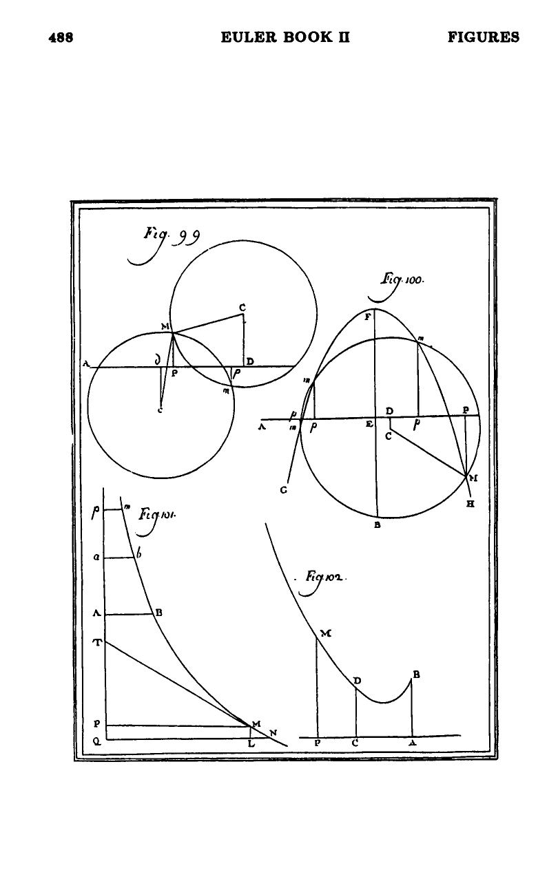
Quadratic by two circles (§492, figure 99)

Two circles also meet in at most 2 points. The construction works algebraically but is less preferred than line + circle: it has six free constants instead of three, the radical-axis derivation is fussier, and circles cannot realize anything beyond a quadratic.

See quadratic-by-two-circles.

Biquadratic by circle and parabola (§§493–495, figure 100)

A circle (order 2) and a parabola (order 2) meet in at most $2\times 2=4$ points. Algebra produces a quartic eliminant which, after the Tschirnhaus shift $z\mapsto z+A/4$ removes the cubic term, leaves the canonical form $z^4+B{z}^2-Cz+D=0$. The parameters of the parabola and circle are determined up to one free length $h$ (the parabola’s parameter), with sign analysis on $D$ showing the construction is always real:

• $D=E^2>0$: explicit choice $h=C/(4E)$, $a=2E^2/C$, etc.
• $D=-E^2<0$: $h$ free, $c$ always real.
• $D\to 0$ (i.e., $E\to 0$): the quartic collapses to the cubic $z^3+Bz-C=0$, handled by Bäcker’s rule.

See biquadratic-by-circle-and-parabola.

2. The intersection degree bound (§§496–498)

Two algebraic curves of orders $m$ and $n$ meet in at most $mn$ points. Euler verifies the bound case by case via the chapter-19 eliminant tables, and also gives a geometric proof: an order-$n$ curve can degenerate (as a complex curve) into $n$ straight lines, each of which meets an order-$m$ curve in at most $m$ points, so the union meets it in $\le nm$ points; by continuity, the bound persists when the order-$n$ curve is irreducible.

$(m,n)$	bound	matches
$(1,n)$	$n$	line + curve, line-curve-intersection-bound
$(2,2)$	$4$	two conics, the biquadratic
$(2,3)$	$6$	conic + cubic
$(3,3)$	$9$	two cubics
$(4,4)$	$16$	two quartics

To construct an equation of degree $N$, choose $mn=N$ (or $mn\ge N$ when $N$‘s factorization is awkward; the surplus $mn-N$ intersections are spurious roots, recognized and discarded). For prime or awkward $N$ — e.g., $N=39$ — choose $m,n$ giving a cleaner product, like $6\cdot 7=42$, rather than the exact but visually intractable $3\cdot 13$.

See intersection-product-degree-bound.

3. The general construction method (§§499–504)

For any equation $\Phi (z)=0$ of any degree, the recipe:

1. Pick the first curve as $P(z)+Q(z)y=0$, so that $y=-P(z)/Q(z)$ is single-valued and rational in $z$. No complex intersections can arise from a curve of this form.
2. Substitute this $y$ into $\Phi (z)=0$ and clear denominators. The result is the equation of the second curve.

The standard worked case is the quartic $z^4+A{z}^3+B{z}^2+Cz+D=0$ with first curve the parabola $ay=z^2+bz$:

$\boxed{a^2{y}^2+a(A-2b)yz+(B-Ab+b^2)z^2+Cz+D=0.}$

The two free constants $a,b$ give an infinite family of valid second curves. The discriminant $A^2-4B-4ac$ (with $c$ added by the §501 trick of multiplying the first equation by $c$) classifies them by conic species: hyperbola / parabola / ellipse. The circle subcase has $b=A/2$ and $c=a+A^2/(4a)-B/a$.

For higher degrees, take the first curve to be a higher-order parabolic line $y=P(z)$ of degree $d$, giving a second curve of order $N/d$. For awkward target degrees, multiply $\Phi$ by $z,z^2,\dots$ to add easily-discarded zero roots — e.g., the cubic $z^3+A{z}^2+Bz+C=0$ becomes the biquadratic $z^4+A{z}^3+B{z}^2+Cz=0$ with $D=0$, ready for the circle-and-parabola construction (and the extra root $z=0$ is the origin).

See general-construction-by-parabola-and-conic.

4. Caveat on missed real roots (§505)

Even when no complex intersections arise (the single-valued first curve ensures this), it can happen that a real root of $\Phi$ corresponds to a point of the second curve that lies off the visible arc — on a different branch, at infinity, or on a part of the curve outside the figure. Euler closes the chapter dismissively: this is “more a curiosity than something useful.”

Connections to the rest of Book II

• The line-curve-intersection-bound from chapter 4 is the $(1,n)$ case of the present $mn$ bound, and the linear construction by two lines is the $(1,1)$ case.
• complex-intersections from chapter 19 motivates the §499 design principle that the first curve be of the form $P+Qy=0$.
• The elimination tables of chapter 19 provide the algebraic engine: each $(m,n)$ table entry tells us the degree of the eliminant, hence the maximum target degree for that pair of construction curves.
• The conic discriminant from chapter 6 sorts the second curves of §502 into hyperbola, parabola, and ellipse.
• The parabola from chapter 6 is the workhorse first curve, both for the biquadratic construction (§§493–495) and for the general parabola+conic method (§§499–504).
• The forward reference: chapter 20 develops the real-affine, multiplicity-free shadow of what becomes Bézout’s theorem in projective complex geometry, where the bound $mn$ becomes an equality.

Figures

Figures 94–98

Figures 99–102

Related pages

• construction-of-equations
• quadratic-by-line-and-circle
• quadratic-by-two-circles
• biquadratic-by-circle-and-parabola
• intersection-product-degree-bound
• general-construction-by-parabola-and-conic
• chapter-19-on-the-intersection-of-curves
• intersection-of-two-curves
• complex-intersections
• elimination-of-ordinate
• line-curve-intersection-bound
• classification-of-conics
• parabola