Coordinate Transformations

Summary: The substitutions by which a curve’s equation in one orthogonal coordinate system is converted to its equation in another. Euler builds them up in stages: translation of the origin along the axis (§§25–26), translation of the axis itself (§§27–28), a right-angle swap of abscissa and ordinate (§§29–30), a rotation about the common origin (§§31–32), and finally the full rigid motion combining translation and rotation (§§33–34).

Sources: chapter2, figures6-10 (figures 7–10), figures11-14 (figure 11)

Last updated: 2026-04-24

---

Why transformations matter (§§23–24)

A curve is defined once its shape is fixed, but its equation depends on two arbitrary choices — the axis $RS$ and the origin $A$ of the abscissas. “Since there are an infinite number of different ways of making these choices, so there are an infinite number of different equations for the same curve” (source: chapter2, §23). The reverse does not hold: different curves always give different equations. Chapter 2 gives the substitutions that carry one valid equation to another, so that the set of all equations for a fixed curve can be generated from any one of them.

Throughout the chapter Euler works with orthogonal coordinates on the curve side; the oblique case is handled separately in oblique-coordinates.

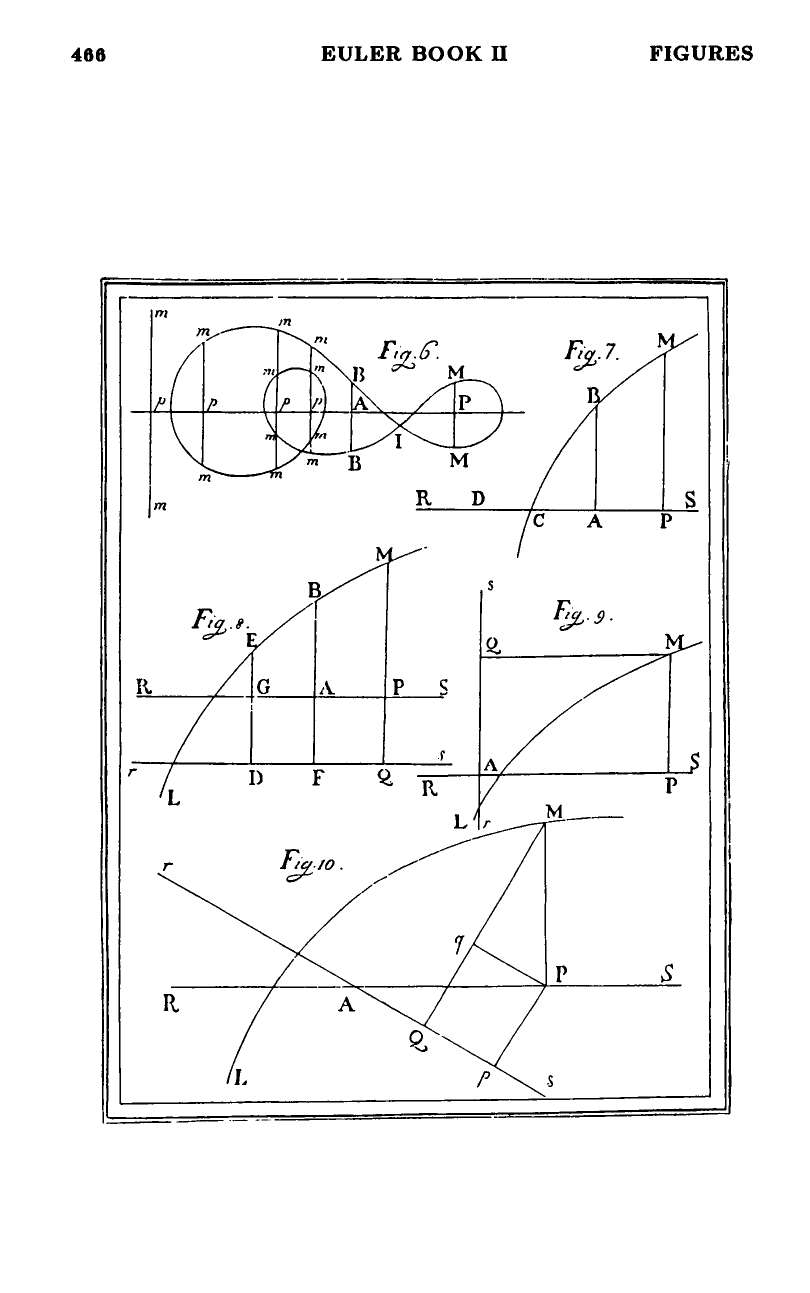
Translation of the origin along the axis (§§25–26)

Same axis $RS$; move the origin from $A$ to a new point $D$ on the same line, with $AD=f$ (figure 7). Let $x=AP$, $y=PM$ be the old coordinates and $t=DP$, $y=PM$ the new. Then

$$t=f+x,x=t-f.$$

Substituting $t-f$ for $x$ in the old equation produces the new equation. The sign convention: $f>0$ when $D$ is to the left of $A$; $f<0$ when $D$ is to the right (§27). Since $f$ is arbitrary, this substitution alone already produces infinitely many equations for the same curve.

A useful corollary (§26): the curve meets the axis precisely where $y=0$, so the intersections with $RS$ are read off by solving the equation with $y$ set to zero. If $C$ is such a point and we take $C$ for origin, the new equation satisfies $y=0$ whenever the abscissa is $0$.

Translation of the axis parallel to itself (§§27–28)

Now shift the axis too: the new axis $RS$ is parallel to the old, at perpendicular distance $AF=g$ from it, and the new origin $D$ is still offset by $AG=f$ along the old axis (figure 8). The new coordinates $t=DQ$, $u=QM$ of the same point $M$ satisfy

$$t=f+x,u=g+y,$$

so

$$x=t-f,y=u-g.$$

Again $f$ and $g$ are arbitrary, so the pair of substitutions produces infinitely many equations for the same curve. “If two equations … differ from each other only in that one can be transformed into the other by increasing or decreasing the coordinates, then both equations, although different, still exhibit the same curve” (source: chapter2, §28).

Swap of abscissa and ordinate (§§29–30)

A new axis $rs$ perpendicular to $RS$, crossing at the same origin $A$ (figure 9). Dropping the perpendicular from $M$ to $rs$ gives the rectangle $APMQ$, so

$$t=AQ=y,u=QM=x.$$

The substitutions are simply to exchange the letters: put $t$ for $y$ and $u$ for $x$ in the old equation. Geometrically the curve has not moved; only our choice of which axis is “horizontal” has flipped. Euler concludes (§29):

The abscissa and ordinate are called coordinates, making no distinction which is called the abscissa or ordinate. Given an equation in $x$ and $y$, the same curve emerges whether $x$ or $y$ is taken as the abscissa.

The sign choices (which half-axis is positive for abscissas, which half-plane is positive for ordinates) are independent and can all be flipped by changing signs in the equation (§30). None of these changes alters the curve.

Rotation of the axes about a common origin (§§31–32)

Common origin $A$; the new axis $rs$ makes an angle $SAs=q$ with the old axis $RS$ (figure 10). Set $\sin q=m$, $\cos q=n$, so that $m^2+n^2=1$. For a point $M$ with old coordinates $AP=x$, $PM=y$, and new coordinates $AQ=t$, $QM=u$, elementary right-triangle decomposition gives

$$\begin{array}{rl}t& =x\cos q-y\sin q=nx-my,\\ u& =x\sin q+y\cos q=mx+ny.\end{array}$$

Inverting (use $m^2+n^2=1$):

$$\boxed{x=mu+nt,y=nu-mt.}$$

Substituting these for $x$ and $y$ in the old equation gives the equation in the new rotated coordinates (§32). The sign of $m$ encodes the direction of the rotation: if the new axis lies above (rather than below) the old, $q$ is negative, so $m$ becomes negative.

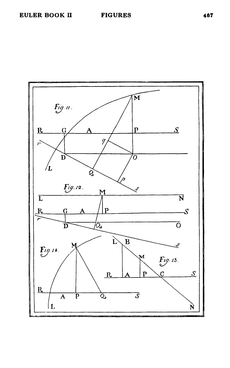
The general rigid motion (§§33–34)

Combine the two moves: the new axis $rs$ is neither parallel to nor passing through the old origin. Drop a perpendicular from the new origin $D$ to the old axis, of length $DG=g$; its foot $G$ lies at $AG=f$ from $A$. The new axis makes angle $ODs=q$ with a line through $D$ parallel to the old axis; set $m=\sin q$, $n=\cos q$ as before (figure 11).

The derivation runs through auxiliary perpendiculars $Op$, $Oq$, $Pp$, $Qq$; the result is the pair

$$t=nx-my+nf-mg,u=mx+ny+mf+ng,$$

which by $m^2+n^2=1$ rearranges to

$$\boxed{x=mu+nt-f,y=nu-mt-g.}$$

These are the substitutions for the most general orthogonal coordinate change. The previous cases are special instances:

Case	Constraints	Recovered formulas
Origin shift along axis (§25)	$g=0,q=0\Rightarrow m=0,n=1$	$x=t-f$, $y=u$
Parallel axis shift (§27)	$q=0$	$x=t-f$, $y=u-g$
Swap of axes (§29)	$f=g=0,q=90^{\circ }\Rightarrow m=1,n=0$	$x=u$, $y=-t$ (or $t$, up to sign convention)
Pure rotation (§31)	$f=g=0$	$x=mu+nt$, $y=nu-mt$

The upshot

Every orthogonal equation for a given plane curve is obtained from any one of them by a suitable choice of the four parameters $f,g,m,n$ (with $m^2+n^2=1$). This is the first half of the chapter’s payoff; the other half — that different equations arising this way still describe the same curve, and can be tested for equivalence — is developed in general-equation-of-a-curve. Oblique coordinates add a fifth parameter (the obliquity angle) and are treated in oblique-coordinates.

Two structural observations fall out for free and are harvested in their own right:

• The degree of the equation is invariant under all these substitutions, since each substitution is first-degree in the new coordinates (§37, §46). See degree-invariance.
• Every first-degree equation, in any orthogonal coordinate system, represents a straight line. See straight-line-equation.

Figures

Figures 6–10

Figures 11–14

Related pages

• chapter-2-on-the-change-of-coordinates
• general-equation-of-a-curve
• degree-invariance
• straight-line-equation
• oblique-coordinates
• abscissa-and-ordinate