appendix-1-on-the-surfaces-of-solids

Appendix Chapter 1 — On the Surfaces of Solids

Summary: Opening chapter of the Appendix on Surfaces. Euler extends Book II’s coordinate apparatus from plane curves to surfaces of solid bodies. Three orthogonal axes give each point of a surface three coordinates $(x,y,z)$; the surface is then characterized by an equation $F(x,y,z)=0$, just as a curve was by $F(x,y)=0$. Single-valued vs. multi-valued, algebraic vs. transcendental, and parity-based reflective and central symmetries are all imported from Book II to the new dimension.

Sources: appendix1, §§1–25. Figures 119, 120 in figures119-120.

Last updated: 2026-05-12.

---

§1 — From plane curves to surfaces

Curves that do not lie in a plane have two kinds of curvature — recently treated by Clairaut — and are inseparable from the surfaces on which they sit. Euler therefore opens this Appendix by treating space curves and surfaces simultaneously.

§§2–3 — Surfaces are to planes as curves are to lines

Surfaces are either planar or non-planar (convex, concave, or mixed). A surface is planar iff every four of its points lie in one plane, just as a curve is straight iff every three of its points lie on one straight line. To investigate a non-planar surface, choose an arbitrary plane and study the perpendicular distance from each point of the surface to it (parallel to how a plane curve is studied via distances to a chosen axis).

§§4–12 — Coordinate apparatus

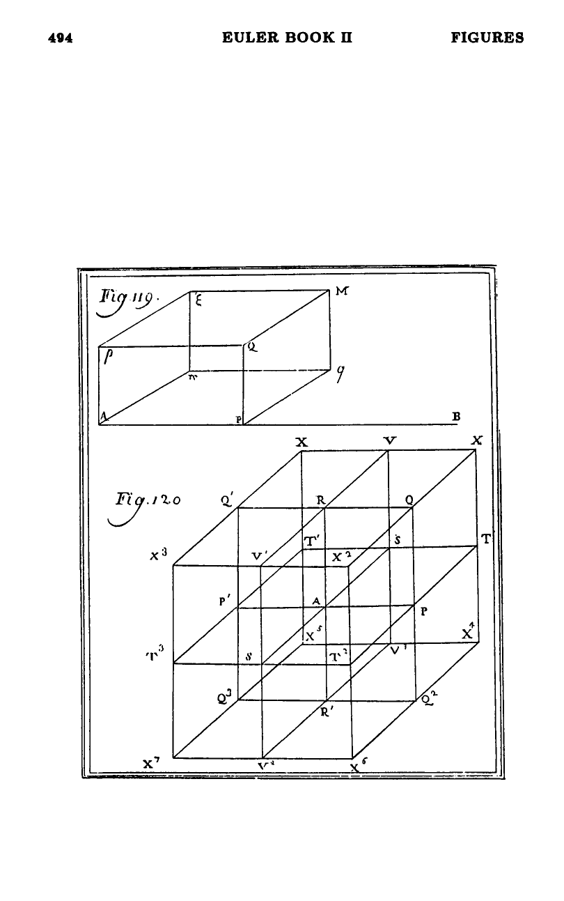
Three perpendicular coordinates $AP=x$, $PQ=y$, $QM=z$ locate any point $M$ in space (figure 119). Three mutually perpendicular planes meet at the origin $A$, and the same surface admits six different coordinate orderings (§10) depending on which plane plays the role of $APQ$ and which axis lies in it. The straight-line distance from $A$ to $M$ is $\sqrt{x^2+y^2+z^2}$.

The surface itself is given by an equation in $x,y,z$; the value of $z$ at each $(x,y)$ records the perpendicular distance from the surface to the chosen plane (positive above, negative below, complex = no point on that perpendicular, multiple = the perpendicular cuts the surface in several points). See surface-coordinates-and-equation.

§§6–7 — First classifications

A continuous (regular) surface is given by a single equation; an irregular surface is patched from several (e.g. a sphere joined to a cone). Among regular surfaces, the principal division is into algebraic and transcendental — exactly the curve dichotomy from chapter 1 of Book II, lifted one dimension up. See algebraic-and-transcendental-surfaces.

§§8–9 — Single-valued vs. multi-valued

If $z=P(x,y)$ with $P$ a single-valued (non-irrational) function, every perpendicular line through $Q$ in the plane $APQ$ meets the surface in a single point — never in a complex number. The next levels are

$$z^2-Pz+Q=0\text{(two real or two complex)},z^3-P{z}^2+Qz-R=0\text{(three or one)},$$

exactly mirroring multi-valued-curves for plane curves.

§§13–14 — Diametral planes

If the equation contains $z$ only with even exponents, the surface has matching parts on either side of the plane $APQ$ — so $APQ$ bisects the solid. Such a plane is called a diametral plane, the surface analogue of a Book II diameter-of-conic (and of the diameter-and-center-from-equation parity calculus). The sphere $x^2+y^2+z^2=a^2$ has all three coordinate planes diametral. See diametral-plane.

§§15–25 — Octants and region symmetries

The three coordinate planes divide space into eight regions (figure 120), labelled $PQR,PQr,PqR,pQR,Pqr,pQr,pqR,pqr$ (§§15–16). Two regions are conjugate if they share a tangent plane (one coordinate sign flipped), disjoint if they share only a tangent line (two flipped), opposite if they share only the point $A$ (all three flipped). Euler tabulates the relationships in §§17–18.

The parity of exponents in the equation governs which regions contain congruent parts of the surface (§§19–25):

• $z$ everywhere of even exponent → 4 pairs of congruent regions (mirror across $APQ$);
• joint degree of $(y,z)$ everywhere even or everywhere odd → another 4 pairs (rotate 180° about an axis);
• all three taken together everywhere even or odd → opposite-region congruence (central symmetry);
• combining several conditions → 4-fold or full 8-fold congruence.

Full development in octants-and-region-symmetries.

Cross-references

• Coordinate setup parallel to abscissa-and-ordinate (Book II Chapter 1).
• Multi-valued reduction parallel to multi-valued-curves.
• Diametral plane is the 3D analogue of diameter-and-center-from-equation (Book II Chapter 15).
• Octant congruence rules parallel to the §§337–343 parity arguments for plane curves with diameters and centers.

Figures

Figures 119–120

Related pages

• surface-coordinates-and-equation
• algebraic-and-transcendental-surfaces
• diametral-plane
• octants-and-region-symmetries
• appendix-2-on-the-intersection-of-a-surface-and-an-arbitrary-plane