Chapter 13: On the Dispositions of Curves

Summary: The local counterpart to chapter 12. To study how a curve behaves near a chosen point $M=(p,q)$, Euler translates the origin to $M$ via $x=p+t$, $y=q+u$ and reads the local picture off the lowest non-vanishing homogeneous form in $(t,u)$. Linear form $At+Bu=0$ → tangent. Quadratic form $C{t}^2+Dtu+E{u}^2=0$ governs double points, with $D^2-4CE$ partitioning them into conjugate point / node / tangent contact. Cubic, quartic, … forms govern triple, quadruple, … points. Synthetically, a curve has a $k$-fold point at $M$ iff its equation has the form $\sum P_i(x-p{)}^{k-i}(y-q{)}^i=0$, which forces order-by-multiplicity inequalities.

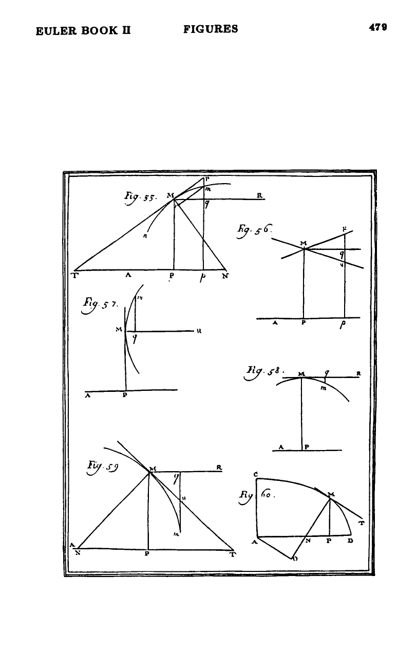
Sources: chapter13 (§§285–302). Figures 55–60 (in figures55-60).

Last updated: 2026-05-07.

---

The motivating analogy (§285)

Just as chapter 7 described the species of branches at infinity by finding straight lines or simpler curves which coincide with the given curve at infinity, this chapter investigates portions of the curve in a bounded region by finding straight lines or simpler curves that coincide with it for at least a small bit. Every tangent is a straight line that has at least two points in common with the curve at the point of tangency. There are also higher-order osculating curves that “kiss” a portion of the given curve more closely.

Strand 1 — tangent by translation (§§286–291)

Take a point $M$ on the curve with $AP=p$, $PM=q$. Substitute $x=p+t$, $y=q+u$ (figure 55). The constant terms cancel because $M$ is on the curve, leaving an equation $0=At+Bu+C{t}^2+Dtu+E{u}^2+F{t}^3+\cdots$ For very small $t,u$, the second- and higher-degree terms are negligible, and the linear truncation $At+Bu=0$ defines a straight line through $M$ — the tangent. See tangent-by-translation.

The inclination ratio $u/t=-A/B$ specializes to figures 57 (when $B=0$, the ordinate $PM$ itself is tangent) and 58 (when $A=0$, the tangent is parallel to the axis).

Strand 2 — subtangent and subnormal (§§289, 292)

From $At+Bu=0$ Euler reads the subtangent $PT=-Bq/A$ and, after dropping the normal at $M$, the subnormal $PN=-Aq/B$ (rectangular coordinates). Normal length $MN=(PM/PT)\sqrt{P{T}^2+P{M}^2}$. Three worked examples — parabola ($PT=2p$, recovering [[parabola|chapter 6’s $PT=2x$]]), ellipse ($PT=-(a^2-p^2)/p$), and a third-order seventh-species cubic ($PT=2p^2{q}^2/(a{p}^2-c)$). See subtangent-and-subnormal.

Strand 3 — singular points by lowest jet (§§293–298)

When $A=B=0$, the tangent is undefined and the second-degree form $C{t}^2+Dtu+E{u}^2=0$ takes over. Three sub-cases by sign of the discriminant:

• $D^2<4CE$: conjugate point (vanishing oval shrunk to a point);
• $D^2>4CE$: node — two distinct real tangent directions, two crossing branches (figure 56);
• $D^2=4CE$: tangent contact (cusp/tacnode in modern terms) — two coincident tangent directions.

If $C,D,E$ also vanish, the cubic form $F{t}^3+G{t}^{2}u+Ht{u}^2+I{u}^3=0$ classifies triple points; quartic form classifies quadruple points; etc. See singular-points-by-jet. This complements multiple-points-on-curves from chapter 12, which arrived at the same taxonomy from the discriminant-collision direction.

Strand 4 — general equation of a curve with a multiple point (§§299–302)

Synthetically, a curve passes through $M$ iff its equation has the form $P(x-p)+Q(y-q)=0$ (with $P,Q$ irreducible against the linear factors). It has a double point at $M$ iff $P(x-p{)}^2+Q(x-p)(y-q)+R(y-q{)}^2=0,$ a triple point iff the equation is homogeneous of degree 3 in $(x-p,y-q)$ with polynomial coefficients, and so on. From these forms Euler reads off order-by-multiplicity ceilings via the chapter-4 line-intersection bound: cubics have at most one double point and no triple points; quartics in Euler’s count at most two double points or one triple; quintuple points need order ≥ 6 in his count; quadruple points need order ≥ 5; two quadruple points need order ≥ 8. (His bound for $r$ doubles on order $n$ is $r\le n-2$, an under-count for $n\ge 4$ relative to the modern Plücker bound $r\le \left(\genfrac{}{}{0ex}{}{n-1}{2}\right)$ — see general-equation-multiple-point.)

Connection to differential calculus (§290)

Euler explicitly notes that the truncate-to-linear method works only when the curve’s equation is non-irrational and free of fractions. For irrational or fractional equations, modifications are needed — and “those modifications give us differential calculus.” This chapter is, in effect, the algebraic prototype of the differential-calculus tangent algorithm.

Figures

Figures 55–60

Related pages

• chapter-12-on-the-investigation-of-the-configuration-of-curves — the dual problem (singular points from discriminant collisions in $x$).
• tangent-by-translation — the master method (§§286–291).
• subtangent-and-subnormal — local rectangular invariants (§§289, 292).
• singular-points-by-jet — multiple-point taxonomy from the lowest jet (§§293–298).
• general-equation-multiple-point — synthetic form for prescribing a $k$-fold point (§§299–302).
• multiple-points-on-curves — chapter 12’s discriminant-collision approach to the same taxonomy.
• line-curve-intersection-bound — the master bound behind every order-by-multiplicity ceiling.
• parabola — §150’s $PT=2x$, recovered as Example I in §289.