Chapter 14: On the Curvature of a Curve

Summary: A second-order extension of chapter 13’s tangent algorithm. After translating origin to a point $M=(p,q)$ on the curve, the linear truncation $At+Bu=0$ gives the tangent. Adding the quadratic terms $C{t}^2+Dtu+E{u}^2$ and rotating to the normal axis gives the osculating parabola, $s^2=(A^2+B^2{)}^{3/2}r/(A^{2}E-ABD+B^{2}C)$. Replacing the parabola with the unique circle of the same vertex-curvature gives the osculating circle, with radius of curvature $R=\frac{(A^2+B^2{)}^{3/2}}{2(A^{2}E-ABD+B^{2}C)}.$ The chapter then handles convexity (sign of the radical), special configurations ($A=0$, $B=0$), a worked ellipse example, the inflection-point classification (when $A^{2}E-ABD+B^{2}C=0$), and curvature at multiple points (cusps and higher-order branches), closing with a three-genus classification of all possible local phenomena and a discussion of L’Hospital’s “cusps of the second species.”

Sources: chapter14 (§§304–335). Figures 55–67 (in figures55-60, figures61-67).

Last updated: 2026-05-11.

---

The motivating analogy (§304)

Just as we have previously investigated straight lines which indicate at a point the direction of a curve, so now we investigate simpler curves which at some place coincide with a given curve so closely that, at least for a very small distance, the two are the same. — §304

Chapter 13 found the tangent line by truncating the local expansion to linear terms. This chapter goes further: keep quadratic terms, get an osculating parabola; replace that parabola by the equally-curved circle, get the osculating circle with its radius of curvature. Higher terms enter only when the second-order data degenerates. The whole program parallels chapter 7’s treatment of branches at infinity, where rectilinear, parabolic, and curvilinear asymptotes refine each other in an analogous hierarchy. See osculating-curves.

Strand 1 — the osculating parabola (§§305–307)

Take the local equation in $(t,u)$ from tangent-by-translation:

$0=At+Bu+C{t}^2+Dtu+E{u}^2+\cdots .$

Rotate to coordinates $(r,s)$ along the normal and tangent at $M$:

$t=\frac{-Ar+Bs}{\sqrt{A^2+B^2}},u=\frac{-As-Br}{\sqrt{A^2+B^2}}.$

Then $r$ is infinitely smaller than $s$ (since $r$ comes out of squares and higher powers of $t,u$). Keeping linear and quadratic terms, the local equation reduces to

$s^2=\frac{(A^2+B^2)\sqrt{A^2+B^2}}{A^{2}E-ABD+B^{2}C}r,$

a parabola with vertex at $M$, axis along the normal, and latus rectum $(A^2+B^2{)}^{3/2}/(A^{2}E-ABD+B^{2}C)$. See osculating-parabola.

Strand 2 — the osculating circle and radius of curvature (§§308–310, §318)

Define the curvature of the given curve at $M$ to equal that of the osculating parabola at its vertex. Replace the parabola by the circle of the same vertex-curvature. Inverting the algorithm on the circle $y^2=2ax-x^2$ gives the conversion: a parabola $s^2=br$ corresponds to a circle of radius $b/2$. Hence the radius of curvature of the original curve at $M$ is

$R=\frac{(A^2+B^2)\sqrt{A^2+B^2}}{2(A^{2}E-ABD+B^{2}C)}.$

This single formula governs the curvature of every algebraic curve at every non-singular point. Its applications (§318): if $R$ is known at every point, the curve can be reconstructed as a chain of small circular arcs. See osculating-circle.

Strand 3 — convexity and special cases (§§311–315)

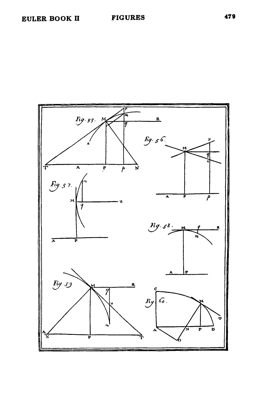
The radius formula is signed only up to the ambiguity of $\sqrt{A^2+B^2}$. Resolving the ambiguity requires asking which side of the tangent the next point lies on. Euler computes the perpendicular drop $w=m\mu$ and finds the sign rule: the curve is concave with respect to $N$ iff $(A^{2}E-ABD+B^{2}C)/B>0$. Two special configurations collapse the formula:

Special case	Tangent direction	Radius
$B=0$ (figure 57)	ordinate $PM$ itself	$A/(2E)$
$A=0$ (figure 58)	parallel to the axis $AP$	$B/(2C)$
general (figures 55, 59)	inclined	$(A^2+B^2{)}^{3/2}/(2(A^{2}E-ABD+B^{2}C))$

See convexity-from-osculating-circle.

Strand 4 — worked ellipse example (§§316–317)

For the ellipse $a^2{y}^2+b^2{x}^2=a^2{b}^2$ at point $(p,q)$:

$A=2b^{2}p,B=2a^{2}q,C=b^2,D=0,E=a^2.$

After applying the constraint $a^2{q}^2+b^2{p}^2=a^2{b}^2$,

$R=\frac{(a^4{q}^2+b^4{p}^2{)}^{3/2}}{a^4{b}^4}=\frac{a^2\cdot M{N}^3}{b^4}=\frac{a^2{b}^2}{M{O}^3}.$

The form $a^2{b}^2/M{O}^3$ is symmetric under exchange of the two axes, with $MO$ the perpendicular from the center to the tangent at $M$ (figure 60). At the major-axis vertex this gives $R=b^2/a$ — half the latus rectum, recovering the classical fact. See osculating-radius-of-ellipse.

Strand 5 — inflection points by vanishing curvature (§§319–322)

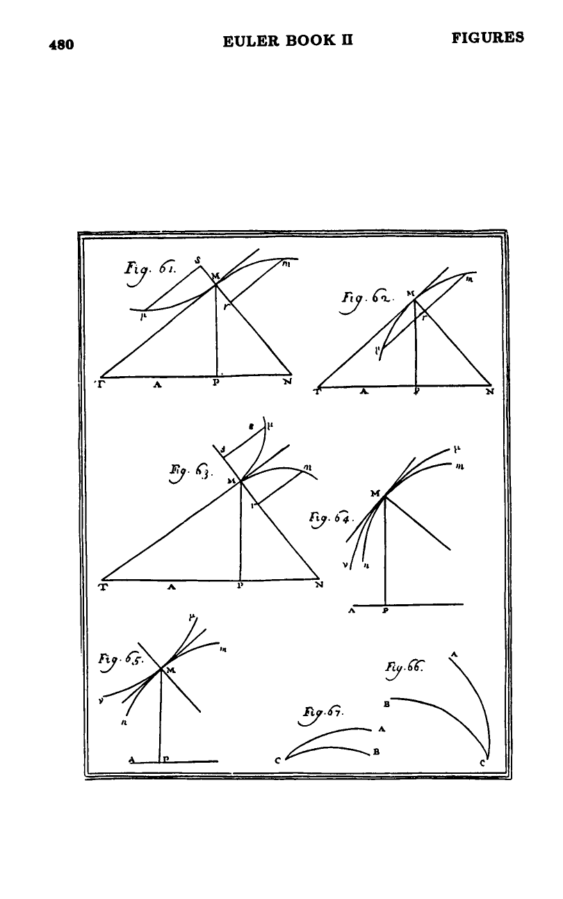
When $A^{2}E-ABD+B^{2}C=0$, the radius is infinite and the osculating circle degenerates to the tangent line. Higher terms decide between an actual inflection (curve crosses through tangent) and a smooth arc just happening to be locally straight to second order. The expansion in the rotated coordinates becomes

$r\sqrt{A^2+B^2}=\alpha s^2+\beta s^3+\gamma s^4+\delta s^5+\cdots .$

The first non-vanishing coefficient gives the answer: odd-power leading term → inflection (figure 61); even-power leading term → both branches on the same side of the tangent, no inflection (figure 62). See inflection-by-vanishing-curvature.

Strand 6 — curvature at multiple points (§§323–331)

When $A=B=0$ ($M$ is a multiple point, figure 56), Euler treats each branch separately. For a branch with its own tangent direction the analysis reduces to the simple-point case — apply the §§319–322 parity rule to that branch’s leading exponent. When two or more branches share a tangent, the local equation has the form

$r^j=\alpha s^n+\cdots$

and the branch is of order $j$. Cases:

• $j=2$, $n=3$: cusp with infinitesimal osculating radius (figure 63).
• $j=2$, $n\ge 5$ odd: cusp with infinite osculating radius.
• $j=2$, branch factors as $r=f{s}^2$ and $r=g{s}^2$: two parabolic-vertex branches; same sign of $f,g$ → internally tangent arcs (figure 64); opposite signs → externally tangent (figure 65).
• general $r^j=\alpha s^n$: odd $j$ behaves like a simple branch; even $j$ produces a cusp; the relation of $n$ to $2j$ controls whether the radius is infinitely small or large.

See curvature-at-multiple-points.

Strand 7 — three-genus master classification (§§332–335)

The phenomena which can occur are reduced to three types. — §332

Genus	Configuration	Osculating radius
1. Continuous curvature	smooth arc, no inflection, no cusp	finite
2. Inflection point	curve crosses through its tangent	infinite or zero, with odd-exponent leading term
3. Cusp / reflex point	two branches mutually tangent	infinite or zero, with even-exponent leading term

Two configurations are explicitly not algebraic: a finite-angle corner (figure 66) and a smooth-cusp where the two tangent branches are one concave / one convex (figure 67). The latter is L’Hospital’s “cusp of the second species,” which Euler initially ruled out but then concedes does occur — as a feature of how branches are paired into continuous arcs when both branches come from the same algebraic equation. The example $y^4-2y^{2}x-4y{x}^2-x^3=0$ (from $y=\sqrt{x}\pm x^{3/4}$) is an explicit fourth-order case. See three-genera-of-local-curvature.

Connection to subsequent chapters

The radius of curvature is the headline quantity that Euler will rely on throughout the rest of Book II for arc-length, surface area, and intersection theory of curves with prescribed local behavior. The §318 picture — “the nature of the curve is seen quite clearly” if $R$ is known at every point — is the geometric content that the Institutiones calculi differentialis will recast as the differential formula $\kappa =y^{\prime \prime }/(1+y^{\prime 2}{)}^{3/2}$.

Figures

Figures 55–60

Figures 61–67

Related pages

• osculating-curves — what “kissing” means.
• osculating-parabola — §§305–307 derivation.
• osculating-circle — §§308–310, §318: the radius formula and its uses.
• convexity-from-osculating-circle — §§311–315: signed analysis.
• osculating-radius-of-ellipse — §§316–317: worked example.
• inflection-by-vanishing-curvature — §§319–322: zero-curvature case.
• curvature-at-multiple-points — §§323–331: cusps and higher-order branches.
• three-genera-of-local-curvature — §§332–335: master classification.
• chapter-13-on-the-dispositions-of-curves — the linear-truncation predecessor.
• singular-points-by-jet — chapter-13 jet classification reused here.