Tangent by Translation

Summary: Euler’s algebraic algorithm for the tangent line to an algebraic curve at a point $M$. Substitute $x=p+t$, $y=q+u$ where $(p,q)=M$; constants cancel because $M$ lies on the curve; collect by total degree in $(t,u)$; keep only the first-degree truncation $At+Bu=0$. As $t,u\to 0$ this straight line through $M$ coincides with the curve, so it is the tangent. The inclination is $u/t=-A/B$. Special cases: $A=0$ → tangent parallel to the axis (figure 58); $B=0$ → ordinate $PM$ is itself the tangent (figure 57).

Sources: chapter13 (§§286–291). Figures 55, 57, 58 (in figures55-60).

Last updated: 2026-05-07.

---

The substitution (§§286–287)

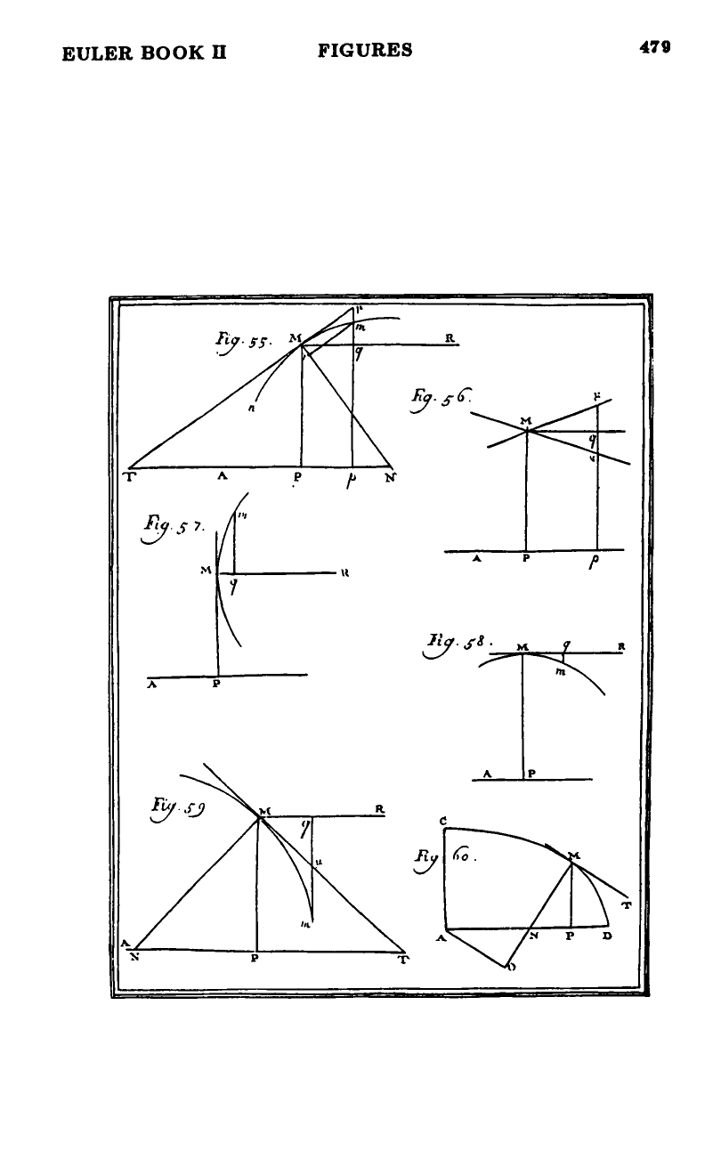
Let $M$ be a point on the curve with abscissa $AP=p$ and ordinate $PM=q$. Through $M$, draw the line parallel to the axis $AP$, taken as a new axis (figure 55). Let $t=Mq$ be the new abscissa along this line and $u=qm$ be the new ordinate, so a generic point near $M$ is $(p+t,q+u)$.

Substitute $x=p+t$, $y=q+u$ into the curve’s equation. Since $M$ lies on the curve, the constant terms cancel. The remaining equation, sorted by total degree in $(t,u)$, takes the form

$0=At+Bu+C{t}^2+Dtu+E{u}^2+F{t}^3+G{t}^{2}u+Ht{u}^2+I{u}^3+\cdots ,$

where the coefficients $A,B,C,D,\dots$ are constants in $p,q$ and the original coefficients of the equation. This is the equation of the curve in the new coordinates, with origin at $M$ and the $t$-axis parallel to the original axis.

Linear truncation (§288)

For the curve’s behavior in a small neighborhood of $M$, take $t,u$ as small as possible. Then $t^2,tu,u^2$ are smaller still; $t^3,t^{2}u,\dots$ smaller yet. So all but the linear terms can be omitted, leaving the equation

$\boxed{At+Bu=0.}$

This is a straight line $M\mu$ through $M$. As $m\to M$ along the curve, $M\mu$ coincides with the curve. Hence $M\mu$ is the tangent to the curve at $M$ (§289).

Why the truncation is legal (§290)

Euler frames a curve as the path of a moving point with continuously changing direction. If the direction did not change at $M$, the line $M\mu$ would describe the curve everywhere; the curve curves precisely because the direction changes. So the tangent records the instantaneous direction at $M$. The linearization captures this direction because as $t,u\to 0$ the higher-degree terms vanish faster than the linear ones.

This is the algebraic prototype of the differential-calculus tangent algorithm. For curves whose equations are irrational or contain fractions, the same idea applies after appropriate modifications — and “those modifications give us differential calculus” (§290).

The inclination ratio (§§289, 291)

From $At+Bu=0$, the slope of the tangent in the new coordinates is

$\frac{u}{t}=-\frac{A}{B}.$

When the original axes are orthogonal, this is also the slope in the original $(x,y)$ coordinates, since the new $t$- and $u$-axes are parallel to the original axes. When the original axes are oblique, the angle $q\mu M$ is fixed by the original obliquity together with the ratio $-A/B$ via plain trigonometry.

Two diagnostic special cases:

• $A=0$: $u/t=0$, so the tangent is parallel to the new $t$-axis — i.e., parallel to the original axis $AP$ (figure 58). The ordinate is at a local extremum.
• $B=0$: the inclination is infinite, so the tangent is parallel to the ordinate direction — that is, the ordinate $PM$ itself is tangent to the curve at $M$ (figure 57).

Algorithm

Given a curve $F(x,y)=0$ and a point $M=(p,q)$ on it, the tangent at $M$ is found by:

1. Substituting $x=p+t$, $y=q+u$ and expanding;
2. Discarding all terms of degree $\ge 2$ in $(t,u)$;
3. Reading the tangent as $At+Bu=0$ in translated coordinates, with slope $-A/B$.

The geometric quantities derived from $A,B$ — subtangent, subnormal, normal length — appear in subtangent-and-subnormal. The case where this algorithm fails because $A=B=0$ at $M$ — meaning $M$ is a singular point — is treated in singular-points-by-jet.

Figures

Figures 55–60

Related pages

• chapter-13-on-the-dispositions-of-curves — chapter summary.
• subtangent-and-subnormal — rectangular invariants $PT=-Bq/A$, $PN=-Aq/B$ derived from this $A,B$.
• singular-points-by-jet — what happens when both $A=0$ and $B=0$ at $M$.
• parabola — §150’s tangent property $PT=2x$, recovered in §289 Example I as the simplest application.