Relations at Symmetric Abscissas

Summary: §§380–390 of chapter-16-on-finding-curves-from-properties-of-the-ordinate. The previous strands related ordinates corresponding to the same abscissa; this strand relates ordinates $PM$ at $AP=z$ and $QN$ at $AQ=-z$ — i.e., at symmetric abscissas. Decomposing the equation $y=X(z)$ into even and odd parts gives the dictionary: $PM+QN$, $PM\cdot QN$, and higher symmetric functions of $(PM,QN)$ are even or odd functions of $z$ in patterns determined by parity. Equal-sum (centered at a point) and equal-product (“alternately equal”) families are derived. §388 unifies them under the invariance principle “equation unchanged under simultaneous $z\mapsto -z$ and $y\mapsto a^2/y$.” §390 tabulates the resulting curves of orders 1, 2, 3.

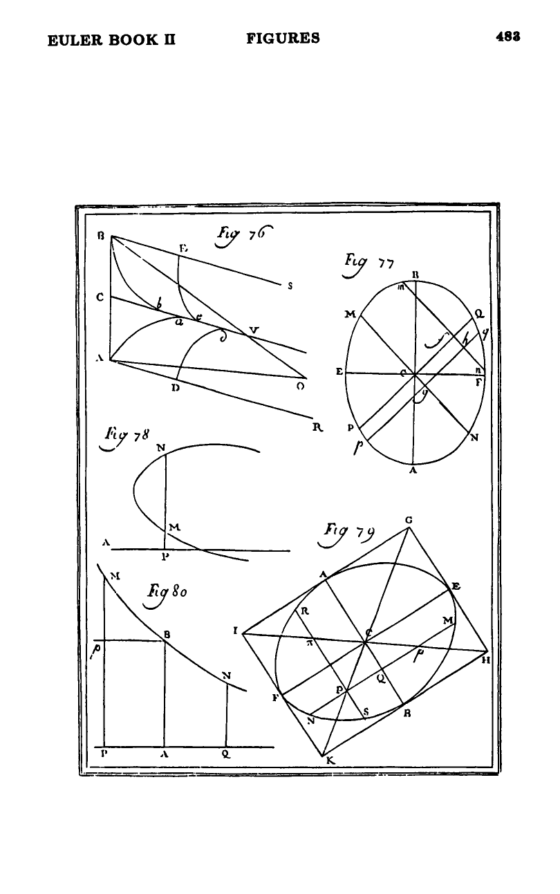
Sources: chapter16 (§§380–390). Figure 80 (in figures76-80).

Last updated: 2026-05-11.

---

The parity dictionary (§380)

For a curve $y=X(z)$ (single-valued for clarity; multi-valued follows analogously), let $PM=X(z)$ at $AP=z$ and $QN=X(-z)$ at $AQ=-z$. Two extreme cases:

Parity of $X$	Relation between $PM$ and $QN$
$X$ even, $X=P(z)$	$QN=PM$ (curve symmetric about the perpendicular through the origin)
$X$ odd, $X=Q(z)$	$QN=-PM$ (curve point-symmetric about the origin)

More generally, decompose $y=(P+Q)/(R+S)$ with $P,R$ even functions of $z$ and $Q,S$ odd. Then

$PM=\frac{P+Q}{R+S},QN=\frac{P-Q}{R-S},$

since flipping the sign of $z$ flips the sign of $Q$ and $S$. Symmetric polynomials of $PM,QN$ split into even-and-odd combinations of $P,Q,R,S$ along the same lines.

Equal-sum: $PM+QN=2a$ (§381)

A curve $MBN$ (figure 80) has center $B$ on the axis if $PM+QN=2a$ for some constant $a$ (equivalent to the midpoint $(PM+QN)/2=a$ being constant). The simplest sufficient form is

$y=a+Q(z)$

with $Q$ an odd function of $z$, giving $PM=a+Q$, $QN=a-Q$ and so $PM+QN=2a$. Geometrically, the curve has equal parts on either side of center $B$, located in opposite quadrants — a $\pi$-rotation symmetry about $B$, the rotational (“alternately equal”) symmetry of diameter-and-center-from-equation.

Letting $u=y-a$ recasts the equation as $u=Q(z)$ with $Q$ odd in $z$ and $u$ odd in $Q$. The two general equations (§382) for curves with rotational symmetry about $B$ in $(z,u)$ coordinates are:

Form I (odd in both $z$ and $u$): $0=\alpha z+\beta u+\gamma z^3+\delta z^{2}u+ϵz{u}^2+\zeta u^3+\eta z^5+\theta z^{4}u+\cdots$

Form II (even constants only, odd-degree mixed terms): $0=\alpha +\beta z^2+\gamma zu+\delta u^2+ϵz^4+\zeta z^{3}u+\eta z^2{u}^2+\theta z{u}^3+\cdots$

Setting $u=y-a$ converts each form into an equation in $(z,y)$ with center at $B$. The form II case includes any central conic (with center at $B$); for the hyperbola, the ordinate $y$ is taken parallel to one asymptote, giving two pairs of ordinates per pair of symmetric abscissas.

Equal $n$th-power sum: $P{M}^n+Q{N}^n=2a^n$ (§383)

The same idea generalized: $y^n=a^n+Q(z)$ with $Q$ odd in $z$. Then $P{M}^n=a^n+Q$, $Q{N}^n=a^n-Q$, and the sum is $2a^n$ for all $z$. Substituting $u=y^n-a^n$ recovers the same forms I and II in $(z,u)$ coordinates.

Equal product: $PM\cdot QN=a^2$ (§§384–386)

Letting $y=P+Q$ with $P$ even and $Q$ odd in $z$, we have $PM=P+Q$, $QN=P-Q$, so $PM\cdot QN=P^2-Q^2=a^2$ requires $P=\sqrt{a^2+Q^2}$. Hence the curve

$y=Q+\sqrt{a^2+Q^2},Q\text{ any odd function of }z.$

The sign ambiguity in the radical gives two ordinates per abscissa, located one positive and one negative — “equal parts alternately placed about $A$ as center.” It is essential that $Q$ not be chosen so that $a^2+Q^2$ is a perfect square (e.g., $Q=a^2/(4z)-z$ gives $\sqrt{a^2+Q^2}=a^2/(4z)+z$, an odd function unfit to be the even $P$), since that would degrade the curve to one ordinate.

The $n$th-power version (§386): $y=(Q+\sqrt{a^{2/n}+Q^2}{)}^n$ with $Q$ odd in $z$ produces $P{M}^n\cdot Q{N}^n=a^{2n}$.

The §387 mixed case

When both $P,R$ are even and $Q,S$ are odd, $y=(P+Q)/(R+S)$ gives $QN=(P-Q)/(R-S)$ and $PM\cdot QN=(P^2-Q^2)/(R^2-S^2)=a^2$. Setting $y=(P+Q)/(P-Q)\cdot a$ or $y=((P+Q)/(P-Q){)}^{n}a$ avoids the radical and ensures only one ordinate per abscissa. The simplest second-order example: $y=(b+z)/(b-z)\cdot a$, a hyperbola.

The §388 unifying invariance principle

The equation for a curve with $PM\cdot QN=a^2$ should be unchanged under the simultaneous substitution $z\mapsto -z$ and $y\mapsto a^2/y$ — the first flips the abscissa to the symmetric one, the second exchanges the two ordinate values whose product is $a^2$. Building blocks invariant under this combined substitution have the form

$\left(y^n-\frac{a^{2n}}{y^n}\right)P(z),\left(y^n+\frac{a^{2n}}{y^n}\right)Q(z)$

with $P$ even in $z$ and $Q$ odd. (The first kind picks up two sign flips and is overall invariant; the second kind picks up no sign flip in the $y^n+a^{2n}/y^n$ factor but a flip in $Q(z)$, so we need the corresponding building block to flip overall — confused; let me state the result Euler actually wrote.) The general equation is:

$0=M+\left(\frac{y}{a}+\frac{a}{y}\right)P+\left(\frac{y^2}{a^2}+\frac{a^2}{y^2}\right)R+\left(\frac{y^3}{a^3}+\frac{a^3}{y^3}\right)T+\cdots +\left(\frac{y}{a}-\frac{a}{y}\right)Q+\left(\frac{y^2}{a^2}-\frac{a^2}{y^2}\right)S+\left(\frac{y^3}{a^3}-\frac{a^3}{y^3}\right)V+\cdots$

with $M,P,R,T,\dots$ any even functions of $z$ and $N,Q,S,V,\dots$ any odd functions. Multiplying through by an odd function of $z$ swaps the role of even and odd, giving a second equivalent general form. Clearing fractions yields (§388 displayed equation):

$0=a^n{y}^{n}M+a^{n-1}{y}^{n+1}(P+Q)+a^{n-2}{y}^{n+2}(R+S)+a^{n-3}{y}^{n+3}(T+V)+\cdots +a^{n+1}{y}^{n-1}(P-Q)+a^{n+2}{y}^{n-2}(R-S)+a^{n+3}{y}^{n-3}(T-V)+\cdots$

and an analogous form II with sign-flips on the lower row.

Fractional exponents (§389)

Substituting $n=1/2,3/2,5/2,\dots$ into the master forms spontaneously eliminates the apparent irrationality, yielding equations such as

$0=\frac{y+a}{(ay{)}^{1/2}}P+\frac{y^3+a^3}{ay(ay{)}^{1/2}}R+\cdots +\frac{y-a}{(ay{)}^{1/2}}Q+\frac{y^3-a^3}{ay(ay{)}^{1/2}}S+\cdots ,$

which after clearing the $(ay{)}^{1/2}$ denominator becomes polynomial in $y$.

Low-order solutions (§390)

The §388 general forms, specialized to low orders, recover concrete curves:

Order	Equation type I (n=1)	Equation type II (n=0)
1 (line)	(vacuous in form I)	(no curve from first eq)
2	$y(\alpha +\beta z)\pm a(\alpha -\beta z)=0$	$\alpha ayz+y^2-a^2=0$ from $N=\alpha z,P=1,Q=0$
3	$ay(\alpha +\beta z^2)+y^2(\gamma +\delta z)+a^2(\gamma -\delta z)$ ; or $\alpha ayz+y^2(\gamma +\delta z)-a^2(\gamma -\delta z)$	$y(\alpha +\beta z+\gamma z^2)\pm a(\alpha -\beta z+\gamma z^2)=0$ ; or $a{y}^2(\alpha +\beta z)+y^3\pm a^{2}y(\alpha -\beta z)\pm a^3=0$

(There is a typographical issue in the printed §390 first-order row: the $n=1$ form-I-first-equation “gives no curves,” and the first explicit curve is the second-order $y=(b+z)/(b-z)\cdot a$ hyperbola. Verified against the §387 derivation.)

The straight line $y=$ const parallel to the axis through $B$ is the trivial order-1 solution. All conics with center at $B$ — including the hyperbola with ordinate parallel to an asymptote — solve the order-2 case. The third-order patterns extend the dictionary.

What this strand really does

Strand 5 is the chapter’s most substantial conceptual contribution. Where strands 1–4 are inverse-direction Newton-identity expansions, strand 5 introduces an invariance group: the cyclic-of-order-2 group generated by $(z,y)\mapsto (-z,a^2/y)$. Building the equation from invariants of that group recovers all “equal product about symmetric abscissas” curves at once. This is exactly the chapter 15 polar-coordinate symmetry analysis (chapter-15-on-curves-with-one-or-several-diameters) recast in rectangular coordinates — a foreshadowing of modern invariant-theoretic curve classification.

Figures

Figures 76–80

Related pages

• chapter-16-on-finding-curves-from-properties-of-the-ordinate — chapter summary.
• diameter-and-center-from-equation — chapter 15 parity-of-exponents version: the same idea for $(x,y)\mapsto (-x,-y)$.
• equal-parts-without-diameter — chapter 15 alternately-equal classification.
• concurrence-of-diameters — chapter 15 angle-quantization version of “equal parts.”
• two-ordinate-sum-and-product — strand 1 same-abscissa counterpart.
• sum-of-ordinate-powers-curves — strand 2 same-abscissa power-sum counterpart.