Osculating Parabola

Summary: §§305–307. The second-order analogue of the tangent line. After [[tangent-by-translation|translating the origin to a point $M$]] on the curve and rotating coordinates so that the new abscissa lies along the normal $MN$ and the new ordinate $rm=s$ is perpendicular to it, Euler keeps the quadratic terms of the local expansion and obtains the osculating equation $s^2=\frac{(A^2+B^2)\sqrt{A^2+B^2}}{A^{2}E-ABD+B^{2}C}r,$ which expresses a parabola with axis along $MN$ and latus rectum $(A^2+B^2{)}^{3/2}/(A^{2}E-ABD+B^{2}C)$. This parabola — the osculating parabola — kisses the curve at $M$, agreeing in tangent direction and in second-order behavior.

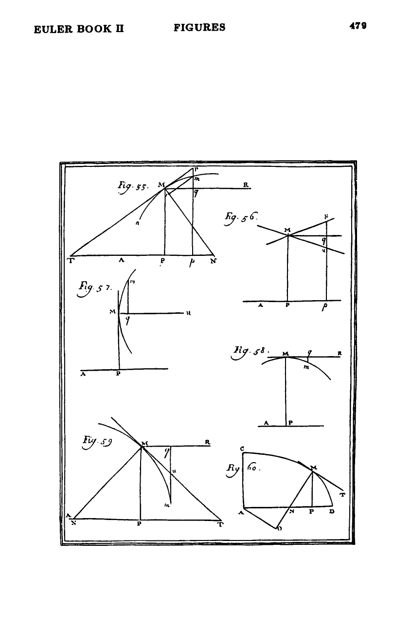
Sources: chapter14 (§§305–307). Figure 55 (in figures55-60).

Last updated: 2026-05-11.

---

Setup: the local equation in $(t,u)$ (§305)

Take the equation of the curve in coordinates $(x,y)$ and pick a point $M$ with $AP=p$, $PM=q$. Substitute $x=p+t$, $y=q+u$ as in tangent-by-translation. Since $M$ lies on the curve the constants drop and we are left with

$0=At+Bu+C{t}^2+Dtu+E{u}^2+F{t}^3+G{t}^{2}u+\cdots ,$

referring to the new axis $MR$ along the original $x$-direction (figure 55). For very small $t,u$ the higher-degree terms are minute compared to the first two and may be neglected without error in the linear approximation.

The tangent line via $(t,u)$ (§306)

Unless both $A$ and $B$ vanish, the linear truncation $At+Bu=0$ defines the tangent $M\mu$ at $M$, with $Mq/q\mu =B/(-A)$. To measure how much the curve $Mm$ deviates from the tangent $M\mu$, Euler introduces the normal $MN$ as the new axis and drops a perpendicular ordinate $mr$ from $m$, with

$Mr=r,rm=s.$

The rotation from $(t,u)$ to $(r,s)$ is an exact rigid rotation through the angle whose tangent is $-A/B$, giving

$$t=\frac{-Ar+Bs}{\sqrt{A^2+B^2}},u=\frac{-As-Br}{\sqrt{A^2+B^2}}.$$

Inversely,

$$r=\frac{-At-Bu}{\sqrt{A^2+B^2}},s=\frac{Bt-Au}{\sqrt{A^2+B^2}}.$$

Now since $-At-Bu=C{t}^2+Dtu+E{u}^2+\cdots$, the quantity $r$ is infinitely smaller than $t$ and $u$, hence infinitely smaller than $s$ as well. (The argument: $s$ is expressed linearly in $t,u$ while $r$ is expressed by squares and higher powers.) This is the key inequality that drives all subsequent estimates.

The osculating equation (§307)

Keep terms up to second order in $(t,u)$:

$-At-Bu=C{t}^2+Dtu+E{u}^2.$

Substitute the rotation formulas for $t$ and $u$ on both sides. The left side is $r\sqrt{A^2+B^2}$. On the right, expansion in powers of $r$ and $s$ gives

$$r\sqrt{A^2+B^2}=\frac{(A^{2}C+ABD+B^{2}E)r^2}{A^2+B^2}+\frac{(A^{2}D-B^{2}D-2ABC+2ABE)rs}{A^2+B^2}+\frac{(A^{2}E-ABD+B^{2}C)s^2}{A^2+B^2}.$$

Because $r$ is infinitely smaller than $s$, the terms in $r^2$ and $rs$ vanish in relation to $s^2$. We are left with

$\boxed{s^2=\frac{(A^2+B^2)\sqrt{A^2+B^2}}{A^{2}E-ABD+B^{2}C}r.}$

This is the equation of the osculating parabola at $M$, in coordinates $(r,s)$ aligned with the normal and tangent at $M$.

Geometric reading (§308)

The equation $s^2=2\ell r$ describes a parabola with axis $MN$ and latus rectum $2\ell$ ([[parabola|chapter 6’s $y^2=2cx$]] with $c=\ell$). Comparing,

$\text{latus rectum}=\frac{(A^2+B^2)\sqrt{A^2+B^2}}{A^{2}E-ABD+B^{2}C}.$

The very short arc $Mm$ of the curve coincides with the vertex of this parabola. Since the parabola’s curvature at its vertex can be matched by a circle of a definite radius, Euler defines the curvature of the given curve at $M$ to be that of the osculating parabola at its vertex. This sets up the osculating circle of the next section.

Why second-order suffices

If only the linear terms are kept, all that is captured is the direction at $M$ — the tangent. To know the curve “much more accurately” near $M$, the second-degree terms must be brought in. Together they fix not only direction but also the bending: a unique parabola tangent to $M\mu$ at $M$ with the same second-order contact. Higher than second order would over-determine — a circle, the standard yardstick of curvature, has only one free parameter (its radius), and that single parameter is what the second-order coefficients pin down.

Worked check: a circle of radius $a$ (§309)

For the circle $y^2=2ax-x^2$, set $AP=p$, $PM=q$ with $q^2=2ap-p^2$, then substitute $x=p+t$, $y=q+u$:

$0=2at-2pt-2qu-t^2-u^2.$

Read off $A=2a-2p$, $B=-2q$, $C=-1$, $D=0$, $E=-1$. Then

$A^2+B^2=4(a-p{)}^2+4q^2=4a^2,$ $A^{2}E-ABD+B^{2}C=-A^2-B^2=-4a^2,$ $\frac{(A^2+B^2)\sqrt{A^2+B^2}}{A^{2}E-ABD+B^{2}C}=\frac{4a^2\cdot 2a}{-4a^2}=-2a,$

so the osculating-parabola equation is $s^2=-2ar$ — a parabola with latus rectum $2a$. The sign indicates the parabola opens toward $-r$, that is, with the curve concave toward $N$. Conversely (Euler’s argument): if a curve has osculating parabola $s^2=br$, its osculating circle has radius $b/2$. The chain $\text{circle}\to \text{parabola}\to \text{circle}$ is consistent.

Figures

Figures 55–60

Related pages

• chapter-14-on-the-curvature-of-a-curve — chapter summary.
• osculating-curves — what “kissing” means; place of the parabola in the program.
• osculating-circle — §§308–310: replace the parabola with a circle of the same vertex-curvature.
• tangent-by-translation — the chapter-13 linear truncation that this construction extends.
• parabola — the canonical $y^2=2cx$ form used here for the osculating curve.
• convexity-from-osculating-circle — sign analysis of $A^{2}E-ABD+B^{2}C$.