Conjugate Diameters

Summary: Two diameters $GI$ and $EF$ of a conic are called conjugate when each bisects all chords parallel to the other (§111). With the center as origin and any diameter as axis, the conic’s equation is $y^2=\alpha -\beta x^2$, and the chord through the center parallel to the ordinates — the diameter $EF$ with $CE=CF=\sqrt{\alpha }$ — is the conjugate of the axis diameter $GI$ with $CG=CI=\sqrt{\alpha /\beta }$. Under any oblique change of coordinates the conjugate-pair structure is preserved (§§112–115), and two metric invariants emerge: the parallelogram circumscribed about any conjugate pair has constant area $fg\sin q$ (§§116–117), and the sum of squares of any pair of conjugate semidiameters is constant, $C{E}^2+C{G}^2=C{K}^2+C{M}^2$ (§§118–120).

Sources: chapter5 §§109–120, figures26-29 (figures 26, 27)

Last updated: 2026-04-25

---

Diameter and conjugate emerge from the center-form equation (§§109–111)

After the center is taken as origin and a diameter as axis, the conic’s equation reduces to (see center-of-conic §§109–110) $y^2=\alpha -\beta x^2.$

Setting $y=0$ gives the endpoints of the diameter on the curve: $x=\pm \sqrt{\alpha /\beta },CG=CI=\sqrt{\alpha /\beta },GI=2\sqrt{\alpha /\beta }.$

Setting $x=0$ gives a chord through the center parallel to the ordinates: $y=\pm \sqrt{\alpha },CE=CF=\sqrt{\alpha }.$

Since $EF$ passes through the center, it is itself a diameter (every chord through the center is a diameter — §107). The chord direction it bisects: by the diameter-construction logic of diameter-of-conic §91, the diameter $EF$ bisects every chord parallel to the original chord direction — i.e., parallel to the original ordinates, which were parallel to $GI$ (the original axis direction)… wait, this needs careful unpacking.

Actually, by symmetry of the equation $y^2=\alpha -\beta x^2$:

• Fix $x$, the chord at that abscissa has ordinates $\pm \sqrt{\alpha -\beta x^2}$, symmetric about $y=0$. So the line $y=0$ (the axis $GI$) bisects every chord at fixed $x$ — i.e., every chord parallel to $EF$.
• Fix $y$, the chord at that ordinate has abscissas $\pm \sqrt{(\alpha -y^2)/\beta }$, symmetric about $x=0$. So the line $x=0$ (the diameter $EF$) bisects every chord at fixed $y$ — i.e., every chord parallel to $GI$.

Each diameter bisects all chords parallel to the other: this is the conjugate property.

These two diameters, $GI$ and $EF$, are related to each other in such a way that one bisects all chords parallel to the other. Because of this reciprocal property, these two diameters are called CONJUGATE. (source: chapter5, §111)

Tangents at the endpoints of a diameter (§111)

The same equation reveals: the tangent at $G$ (where $y$ is “extremal” as $x\to CG$) is parallel to $EF$, and the tangent at $E$ is parallel to $GI$. More generally, the tangent at the endpoint of any diameter is parallel to the conjugate diameter.

This is the coordinate-free statement: pick any diameter; the tangents at its two endpoints on the curve are both parallel to the conjugate diameter.

Oblique change of variables preserves conjugacy (§§112–115)

Take any oblique ordinate $MQ$ at angle $\angle AQM=\varphi$ to the axis, with $\sin \varphi =\mu$, $\cos \varphi =\nu$. New coordinates: $CQ=t$, $QM=u$. Trigonometry on triangle $PMQ$ (where $\angle PMQ=\varphi -q$ with $q$ = original axis–ordinate angle) gives $y=\mu u/m,x=t-(\mu n-\nu m)u/m,$ where $\sin q=m$, $\cos q=n$. Substituting into $y^2+\beta x^2-\alpha =0$: $({\mu }^2+\beta (\mu n-\nu m{)}^2)u^2-2\beta m(\mu n-\nu m)tu+\beta m^2{t}^2-\alpha m^2=0.$

The new diameter for chords parallel to $QM$ has the equation (sum of $u$-roots = $2v$ for midpoint at $Q\ell =v$): $Qp=\frac{\beta m(\mu n-\nu m)t}{{\mu }^2+\beta (\mu n-\nu m{)}^2}.$

So $C\ell p$ is a straight line through $C$ — confirming that every chord through the center is a diameter, in any oblique system (no surprise; just verifies §107).

Now compute the semidiameter lengths $a=CG=$ half the diameter parallel to $QM$ direction (i.e., setting $u=0$? No, setting that direction as new axis); and $b=CE=$ semiconjugate.

After algebra (§§114–115): $a=f\sqrt{\frac{\sin q\sin (q+\pi )}{\sin (q-p)\sin (q+\pi -p)}},b=g\sqrt{\frac{\sin q\sin (q-p)}{\sin (q+\pi )\sin (q+\pi -p)}}$ where $\angle GCe=p$ is the angle between the new diameter $Cg$ and the old conjugate $CE$, $\angle ECG=q$ is the angle between the old conjugate pair, and $\pi$ is short for the angle $\angle ECe$ (so $\sin \pi$ is not zero — it’s $\sin (\angle ECe)$, an unfortunate notational collision in Euler’s text).

These are the lengths of the new conjugate pair in terms of the old conjugate pair. The pair $(a,b)$ is also conjugate — the conjugate-pair structure transforms covariantly.

Equal parallelograms (§§116–117)

From the formulas above, $ab=\frac{fg\sin q}{\sin (q+\pi -p)}.$

Rearranging, $ab\sin (q+\pi -p)=fg\sin q.$

Now, $q+\pi -p$ is the angle at the center between the new conjugate pair $a,b$, and $q$ is the angle between the old conjugate pair $f,g$. The product $a\cdot b\cdot \sin (\text{angle between})$ is the area of the parallelogram with sides $a$ and $b$ — equivalently, twice the area of the triangle with vertices at the center and at the endpoints of the two semidiameters.

$\text{Area of parallelogram on conjugate pair }(a,b)=\text{Area of parallelogram on conjugate pair }(f,g).$

Geometrically: if we double each conjugate pair into a full diameter pair $GI,EF$ (or $gi,ef$) and circumscribe the parallelogram tangent to the conic at each endpoint (tangent at $G$ is parallel to $EF$, etc., by §111), the resulting parallelogram has area $4ab\sin (\text{angle})=4fg\sin q$. So:

All parallelograms which are described around the pairs of conjugate diameters are equal to each other. (source: chapter5, §116)

This is one of the two classical metric invariants of a conic with a center.

Sum of squares of conjugate semidiameters (§§118–120)

Set $\angle GCE=q$, $\angle GCM=p$, $\angle ECK=\pi$ (Euler’s notation, again collision-prone). From §119, after applying sum-to-product identities, $\frac{C{E}^2+C{G}^2}{C{G}^2}=\frac{C{K}^2+C{M}^2}{C{M}^2}\cdot \frac{C{G}^2}{C{M}^2}\cdot \frac{C{M}^2}{C{G}^2}=\frac{\sin q\sin (p+\pi )}{\sin \pi \sin (q-p)}\cdot \dots$

After simplification (a sequence of trig identities including $\sin A\sin B=\frac{1}{2}[\cos (A-B)-\cos (A+B)]$):

$\frac{C{E}^2+C{G}^2}{C{K}^2+C{M}^2}=\frac{C{G}^2}{C{M}^2}\cdot \frac{\sin q\sin (q+\pi )}{\sin (q-p)\sin (q+\pi -p)}=\frac{C{G}^2}{C{M}^2}\cdot \frac{C{M}^2}{C{G}^2}=1.$

Hence $C{E}^2+C{G}^2=C{K}^2+C{M}^2.$

In any second order line the sum of the squares of two conjugate semidiameters is always constant. (source: chapter5, §119)

This is the second classical metric invariant.

Practical use of the invariants (§120)

Given two conjugate semidiameters $CG,CE$ and any other semidiameter $CM$, the conjugate $CK$ to $CM$ is computable: $CK=\sqrt{C{E}^2+C{G}^2-C{M}^2}.$

This will be used in principal-axes-and-foci to find the orthogonal conjugate pair (the unique one for which the angle between them is a right angle).

Tangent construction at a general point (§118, figure 27)

Given conjugate semidiameters $CG,CE$, choose any point $M$ on the curve and form $MP$ parallel to $CE$ to the axis (so $PM$ is a semichord parallel to $CE$, with $PN=PM$). The tangent at $M$ is parallel to the conjugate semidiameter $CK$ where $C{K}^2=C{E}^2+C{G}^2-C{M}^2.$

Hence the tangent direction is constructable from $CM$ and the conjugate-pair sum of squares.

This is more than a curiosity — it is the construction of a tangent to a conic at any of its points using only the conjugate semidiameters, no calculus needed. It will lead in §§121–124 to the Newton tangent ratios.

The dual reading of $y^2=\alpha -\beta x^2$

The reduced form $y^2=\alpha -\beta x^2$ has two coefficients $\alpha ,\beta$ that admit two interpretations:

• Diameter-and-conjugate reading. $\sqrt{\alpha }$ = semiconjugate, $\sqrt{\alpha /\beta }$ = semidiameter on the chosen axis.
• Coefficient reading. $\alpha$ controls the “size” of the conic; $\beta$ controls its eccentricity along the chosen axis.

When $\beta >0$, both semidiameters are real — the conic is closed (an ellipse). When $\beta <0$, the axis-semidiameter is imaginary — Euler will read this as the curve having no real intersection with the axis (a hyperbola in disguise). The case-split is classified in chapter 6 by the sign of the discriminant.

Why “conjugate”?

The relationship is reciprocal: $GI$ bisects chords parallel to $EF$ and $EF$ bisects chords parallel to $GI$. Each plays the same role for the other. This is unlike the diameter-chord pairing in general, where the diameter sits on one side and “the chord direction” on the other; for conjugate diameters, both lines are simultaneously diameters and both are simultaneously chord-directions for each other.

Algebraically, conjugacy expresses the symmetry of the equation $y^2=\alpha -\beta x^2$ under each of $x\to -x$ and $y\to -y$ separately, plus the swap $x\leftrightarrow y$ when $\alpha =\beta$ (giving the circle, where every diameter is its own conjugate’s mirror — see principal-axes-and-foci §127).

Figures

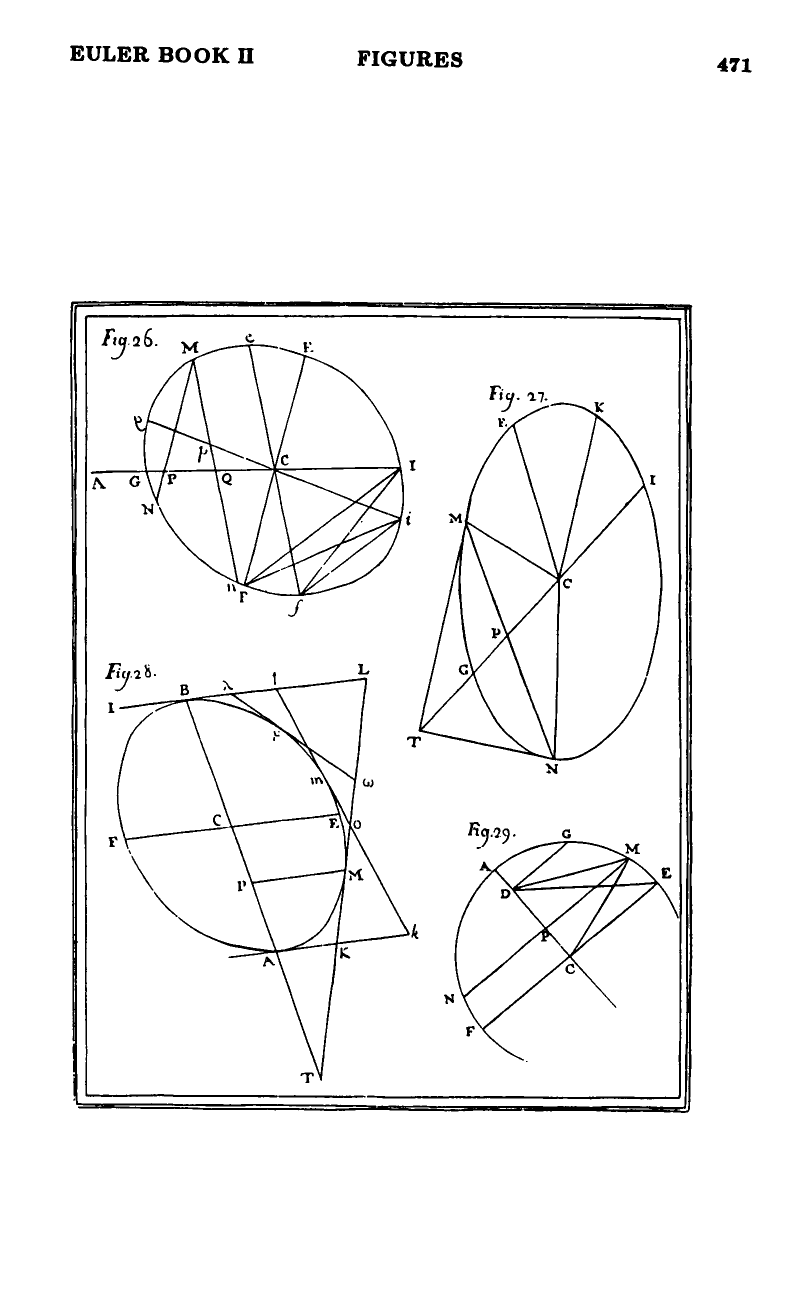Figures 26–29

Related pages

• chapter-5-on-second-order-lines
• center-of-conic — every diameter passes through the center; the center is the origin for the reduced equation
• diameter-of-conic — definition of diameter as bisector of parallel chords
• principal-axes-and-foci — exactly one conjugate pair is orthogonal
• tangent-properties-conic — tangent construction at any point uses the conjugate pair
• chord-rectangle-property — companion algebraic strand (product of roots)